sp <- c("wt-rep1","wt-rep2","sgeIF5A-rep1","sgeIF5A-rep2")
gp <- c("wt","wt","sgeIF5A","sgeIF5A")

ribobams <- c("WT.1.sorted.bam","WT.2.sorted.bam","eIF5Ad.1.sorted.bam","eIF5Ad.2.sorted.bam")

obj0 <- construct_ribotrans(genome_file = "../../index-data/Saccharomyces_cerevisiae.R64-1-1.dna.toplevel.fa",
                            gtf_file = "../../index-data/Saccharomyces_cerevisiae.R64-1-1.112.gtf",
                            mapping_type = "genome",
                            assignment_mode = "end5",
                            extend = TRUE,
                            extend_upstream = 50,
                            extend_downstream = 50,
                            Ribo_bam_file = ribobams,
                            Ribo_sample_name = sp,
                            RNA_sample_group = gp,
                            choose_longest_trans = T)

# generate summary data for QC or other analysis
obj0 <- generate_summary(object = obj0, exp_type = "ribo", nThreads = 40)


head(obj0@summary_info)
#               rname  pos qwidth count  sample sample_group mstart mstop translen
# 1 YAL067C_mRNA|SEO1 1774     27     1 wt-rep1      wt-rep1     51  1829     1882
# 2 YAL067C_mRNA|SEO1 1771     27     1 wt-rep1      wt-rep1     51  1829     1882
# 3 YAL067C_mRNA|SEO1 1766     20     1 wt-rep1      wt-rep1     51  1829     1882
# 4 YAL067C_mRNA|SEO1 1761     27     1 wt-rep1      wt-rep1     51  1829     1882
# 5 YAL067C_mRNA|SEO1 1662     28     1 wt-rep1      wt-rep1     51  1829     1882
# 6 YAL067C_mRNA|SEO1 1632 25 1 wt-rep1 wt-rep1 51 1829 1882Pausing site detection
Intro
Ribosome pausing refers to the temporary slowing or stalling of ribosome elongation during protein synthesis, which can be detected through ribosome profiling (Ribo-seq) by identifying abnormally high peaks of ribosome footprint density. These pauses represent sites where ribosomes experience slower elongation rates compared to their local context. To systematically identify ribosome pausing events, we employed the computational approach described by PausePred and Rfeet, specialized webtools designed for inferring ribosome pauses and visualizing footprint density from ribosome profiling data.
The calculation formula shows here:
\[S_i = \frac{n}{2} r_i \cdot \frac{\sum_{i=1}^n r_i + \sum_{i=\frac{n}{2}}^{\frac{3n}{2}} r_i}{\sum_{i=1}^n r_i \cdot \sum_{i=\frac{n}{2}}^{\frac{3n}{2}} r_i}\]
Pausing site detection
Here we still use the previous yeast eif5a ribo-seq data as an example, and we construct objects for the aligned BAM files:
We assign p-site position to adjust mapped reads:
offset <- rbind(data.frame(list(sample = "sgeIF5A-rep1",
                                qwidth = 25:32,
                                rel_pos = -12)),
                data.frame(list(sample = "sgeIF5A-rep2",
                                qwidth = 25:32,
                                rel_pos = -12)),
                data.frame(list(sample = "wt-rep1",
                                qwidth = 25:32,
                                rel_pos = -12)),
                data.frame(list(sample = "wt-rep2",
                                qwidth = 25:32,
                                rel_pos = -12))
)

obj0@reads_offset_info <- offset
Use the get_pausing_sites function to calculate, here we select replicate 1 sample for calculation:
# pause site
# get pause site
ps <- get_pausing_sites(object = obj0,
                        do_offset_correct = T,
                        sample_selected = c("wt-rep1","sgeIF5A-rep1"))

# check
head(ps)
# # A tibble: 6 × 16
# # Groups:   rname, sample [1]
#   rname  relst sample normsm total_counts sum_1 sum_2 pause_score total_sum min_sum max_sum balance_score imbalance_ratio pause_mean
#   <chr>  <dbl> <chr>   <dbl>        <dbl> <dbl> <dbl>       <dbl>     <dbl>   <dbl>   <dbl>         <dbl>           <dbl>      <dbl>
# 1 Q0250…     1 sgeIF…      0            0  56.2  174.           0      230.    56.2    174.         0.244             3.1       1.40
# 2 Q0250…     2 sgeIF…      0            0  56.2  174.           0      230.    56.2    174.         0.244             3.1       1.40
# 3 Q0250…     3 sgeIF…      0            0  56.2  174.           0      230.    56.2    174.         0.244             3.1       1.40
# 4 Q0250…     4 sgeIF…      0            0  56.2  174.           0      230.    56.2    174.         0.244             3.1       1.40
# 5 Q0250…     5 sgeIF…      0            0  56.2  174.           0      230.    56.2    174.         0.244             3.1       1.40
# 6 Q0250…     6 sgeIF…      0            0  56.2  174.           0      230.    56.2    174.         0.244             3.1       1.40
# # ℹ 2 more variables: pause_sd <dbl>, z_score <dbl>

# plot
ps.ft <- ps %>%
  dplyr::filter(pause_score > 20 & z_score > 0)

# check
head(ps.ft)
# # A tibble: 6 × 16
# # Groups:   rname, sample [1]
#   rname  relst sample normsm total_counts sum_1 sum_2 pause_score total_sum min_sum max_sum balance_score imbalance_ratio pause_mean
#   <chr>  <dbl> <chr>   <dbl>        <dbl> <dbl> <dbl>       <dbl>     <dbl>   <dbl>   <dbl>         <dbl>           <dbl>      <dbl>
# 1 Q0250…   559 sgeIF…   5.62          134  191.  28.1        22.9      219.    28.1    191.         0.128            6.8        1.40
# 2 Q0250…   562 sgeIF…  16.9           134  185.  28.1        69.1      214.    28.1    185.         0.132            6.6        1.40
# 3 Q0250…   568 sgeIF…  11.2           268  169.  28.1        46.7      197.    28.1    169.         0.143            6          1.40
# 4 Q0250…   588 sgeIF…  11.2           268  157.  22.5        57.1      180.    22.5    157.         0.125            7          1.40
# 5 Q0250…   591 sgeIF…   5.62          134  146.  16.9        37.2      163.    16.9    146.         0.103            8.67       1.40
# 6 Q0250…   593 sgeIF…  16.9           268  140.  16.9       112        157.    16.9    140.         0.107            8.33       1.40
# # ℹ 2 more variables: pause_sd <dbl>, z_score <dbl>
The original paper showed that 3 genes exhibited significant pausing:
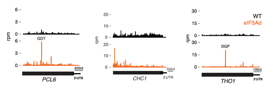
Let’s reproduce these few and take a look, then also mark out the positions where pause_score > 20:
library(ggplot2)

# examples
ps.ft.pt <- ps %>%
  dplyr::filter(rname %in% c("YGL206C_mRNA|CHC1","YER063W_mRNA|THO1",
                             "YER059W_mRNA|PCL6"))

id <- unique(ps.ft.pt$rname)

# loop plot
# x = 1
lapply(seq_along(id),function(x){
  tmp <- subset(ps.ft.pt, rname == id[x])
  tmp.ps <- subset(ps.ft.pt, rname == id[x]) %>%
    dplyr::filter(pause_score > 20 & z_score > 0)

  ggplot(tmp) +
    geom_col(aes(x = relst,y = normsm),fill = "#1A2A80",color = "#1A2A80") +
    geom_point(data = tmp.ps,aes(x = relst, y = 0),
               color = "black",fill = "#FFD700",
               shape = 21,size = 3) +
    # facet_wrap(~sample,scales = "free") +
    ggh4x::facet_grid2(sample~rname,scales = "fixed") +
    theme(panel.grid = element_blank(),
          axis.text = element_text(colour = "black"),
          aspect.ratio = 0.6,
          strip.text = element_text(face = "bold",size = rel(1))) +
    xlab("Position along CDS (nt)") +
    ylab("Ribosome density")
}) -> p

cowplot::plot_grid(plotlist = p,nrow = 1)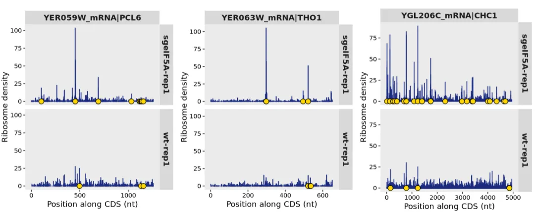
Other pausing genes:
# examples
ps.ft.pt <- ps %>%
  dplyr::filter(rname %in% c("YAL001C_mRNA|TFC3","YGR097W_mRNA|ASK10",
                             "YLR339C_mRNA|YLR339C_mRNA","YDR154C_mRNA|YDR154C_mRNA"))

id <- unique(ps.ft.pt$rname)

# loop plot
# x = 1
lapply(seq_along(id),function(x){
  tmp <- subset(ps.ft.pt, rname == id[x])
  tmp.ps <- subset(ps.ft.pt, rname == id[x]) %>%
    dplyr::filter(pause_score > 20)

  ggplot(tmp) +
    geom_col(aes(x = relst,y = normsm),fill = "#1A2A80",color = "#1A2A80") +
    geom_point(data = tmp.ps,aes(x = relst, y = 0),
               color = "black",fill = "#FFD700",
               shape = 21,size = 3) +
    # facet_wrap(~sample,scales = "free") +
    ggh4x::facet_grid2(sample~rname,scales = "fixed") +
    theme(panel.grid = element_blank(),
          axis.text = element_text(colour = "black"),
          aspect.ratio = 0.6,
          strip.text = element_text(face = "bold",size = rel(1))) +
    xlab("Position along CDS (nt)") +
    ylab("Ribosome density")
}) -> p

cowplot::plot_grid(plotlist = p,nrow = 1)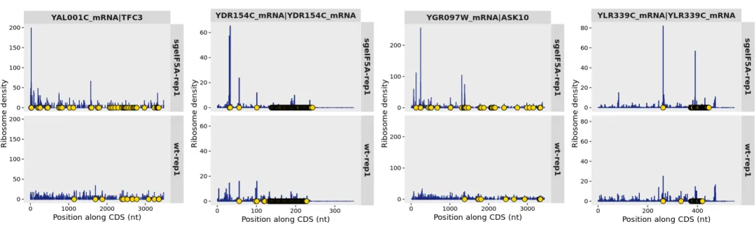
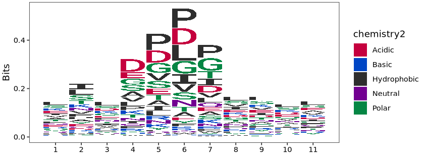
Pausing motif analysis
Pausing sites are often related to the characteristics of flanking sequences, such as the properties of amino acids with different polarities. We can extract motifs around pausing sites to examine the sequence features of the flanking regions.
Here we extract the top 3 pausing sites from each gene, then compare them with wild type to filter for pausing site information that is upregulated in EIF5A knockdown:
# long to wide
ps.wd <- ps %>%
  dplyr::select(rname,relst,sample,z_score,pause_score) %>%
  tidyr::pivot_wider(names_from = sample,values_from = c(z_score,pause_score))

# filter top pause site for each gene and up regulated sites
ps.wd.ft <- ps.wd %>%
  dplyr::filter(`pause_score_sgeIF5A-rep1` > 0 & `pause_score_wt-rep1` > 0) %>%
  dplyr::mutate(ps_ratio = log2(`pause_score_sgeIF5A-rep1`/`pause_score_wt-rep1`),
                zs_ratio = log2(`z_score_sgeIF5A-rep1`/`z_score_wt-rep1`)) %>%
  dplyr::filter(ps_ratio > 1 & zs_ratio > 1) %>%
  dplyr::ungroup() %>%
  dplyr::slice_max(order_by = ps_ratio,n = 3,by = rname)

# check
head(ps.wd.ft)
# # A tibble: 6 × 8
#   rname             relst `z_score_sgeIF5A-rep1` `z_score_wt-rep1` pause_score_sgeIF5A-rep…¹ `pause_score_wt-rep1` ps_ratio zs_ratio
#   <chr>             <dbl>                  <dbl>             <dbl>                     <dbl>                 <dbl>    <dbl>    <dbl>
# 1 YAL001C_mRNA|TFC3  1575                  18.1              1.70                      103.                   6.58     3.96     3.42
# 2 YAL001C_mRNA|TFC3    21                  13.3              1.28                       75.4                  5.24     3.85     3.37
# 3 YAL001C_mRNA|TFC3  1758                   8.49             0.895                      48.7                  3.99     3.61     3.25
# 4 YAL002W_mRNA|VPS8   144                   3.57             0.402                      18.6                  2.76     2.75     3.15
# 5 YAL002W_mRNA|VPS8  2076                  10.6              1.87                       53                    9        2.56     2.51
# 6 YAL002W_mRNA|VPS8   729                   6.66             1.36                       33.7                  6.83     2.30     2.29
# # ℹ abbreviated name: ¹`pause_score_sgeIF5A-rep1`
The get_codon_from_site function can extract surrounding amino acid sequences from the pausing site information filtered above. The left_extend and right_extend parameters specify how many amino acids to extend upstream and downstream:
# get codons around P-sie
pep.df <- get_codon_from_site(object = obj0,
                              cds_fa = "sac_cds.fa",
                              pause_data = ps.wd.ft,
                              left_extend = 5,
                              right_extend = 5)
# check
head(pep.df)
#               rname codon_pos  lp  rp  len        seqs
# 1 YAL001C_mRNA|TFC3       526 521 531 1161 KSAEDSPSSNG
# 2 YAL001C_mRNA|TFC3         8   3  13 1161 LTIYPDELVQI
# 3 YAL001C_mRNA|TFC3       587 582 592 1161 KYMGSTTTLDK
# 4 YAL002W_mRNA|VPS8        49  44  54 1275 YTAPPLNEDGP
# 5 YAL002W_mRNA|VPS8       693 688 698 1275 GFSIKWPSNSN
# 6 YAL002W_mRNA|VPS8       244 239 249 1275 KILDVNSSKEK
Plot motif features, where positions 5-6-7 correspond to EPA sites:
# motif plot
logo_plot(foreground_seqs = pep.df$seqs,
          method = "bits")