Chapter 3 geom_jjboxplot
I re-write the geom_boxplot based on my knowledge and I also add more parameters to control the graphs to be plot. The following shows the details.
3.1 basic plot
load test data first:
library(ggplot2)
library(jjPlot)

# load test data
data("ToothGrowth")

colnames(ToothGrowth)
# [1] "len"  "supp" "dose"
we can show the difference between the geom_jjboxplot and geom_boxplot:
pm <-
  ggplot(ToothGrowth,aes(x = factor(dose),y = len)) +
  geom_jjboxplot(aes(fill = factor(dose)))

pn <-
  ggplot(ToothGrowth,aes(x = factor(dose),y = len)) +
  geom_boxplot(aes(fill = factor(dose)))

cowplot::plot_grid(pm,pn,align = 'hv')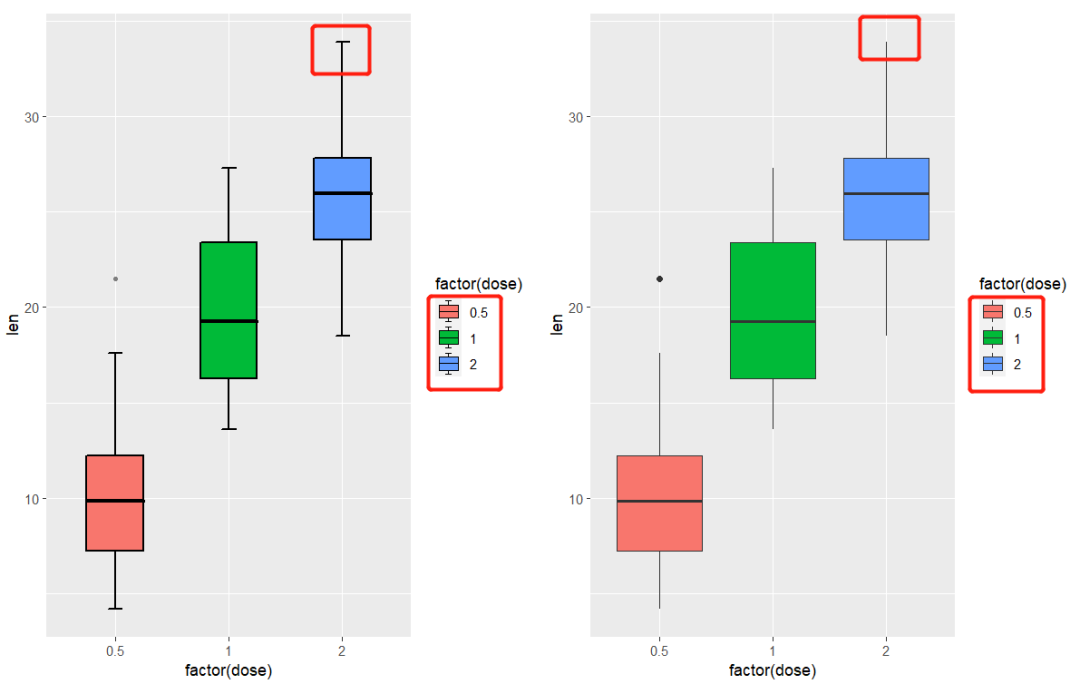
as you can see, I add a small segment on 1.5IQR line and in the legend.
you can also control the outlier points:
ggplot(ToothGrowth,aes(x = factor(dose),y = len)) +
  geom_jjboxplot(aes(fill = factor(dose)),
                 outlier.color = 'black',
                 outlier.size = 5)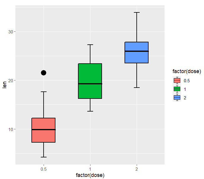
here I supply a parameter(outlier.show) to remove the outlier points:
ggplot(ToothGrowth,aes(x = factor(dose),y = len)) +
  geom_jjboxplot(aes(fill = factor(dose)),
                 outlier.show = F)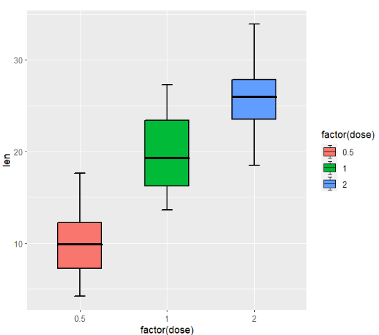
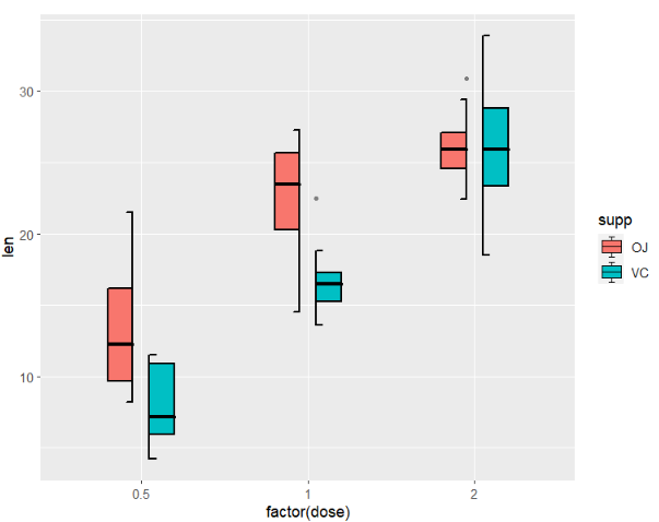
we can use position_dodge to ajust group space:
ggplot(ToothGrowth,aes(x = factor(dose),y = len)) +
  geom_jjboxplot(aes(fill = supp),
                 width = 0.8,
                 position = position_dodge(width = 1))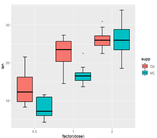
here shows the multiple groups difference:
p3 <-
  ggplot(ToothGrowth,aes(x = supp,y = len)) +
  geom_jjboxplot(aes(fill = factor(dose)),
                 width = 0.6,
                 position = position_dodge(width = 0.75))

p3n <-
  ggplot(ToothGrowth,aes(x = supp,y = len,
                         fill = factor(dose))) +
  geom_boxplot()

cowplot::plot_grid(p3,p3n,align = 'hv')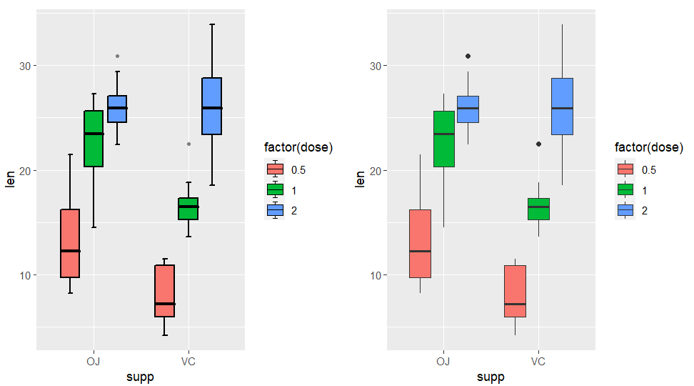
3.2 split boxplot
I supply four types to show the boxplot including full, split, left and right which can make boxplot more flexible for you.
full type(default mode):
ggplot(ToothGrowth,aes(x = factor(dose),y = len)) +
  geom_jjboxplot(aes(fill = factor(dose)),
                 type = 'full')
left type:
ggplot(ToothGrowth,aes(x = factor(dose),y = len)) +
  geom_jjboxplot(aes(fill = factor(dose)),
                 type = 'left')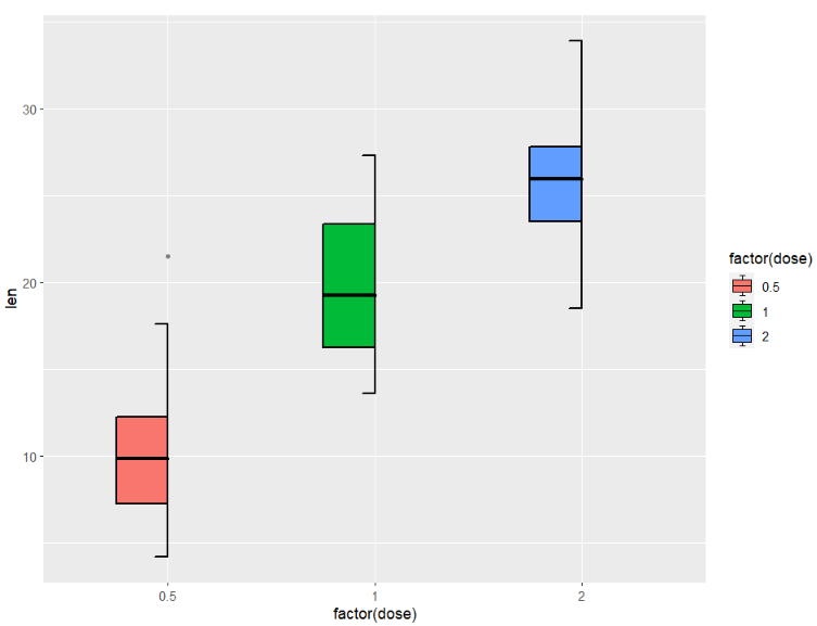
we can use shift to ajust the position:
ggplot(ToothGrowth,aes(x = factor(dose),y = len)) +
  geom_jjboxplot(aes(fill = factor(dose)),
                 type = 'left',
                 shift = -0.05)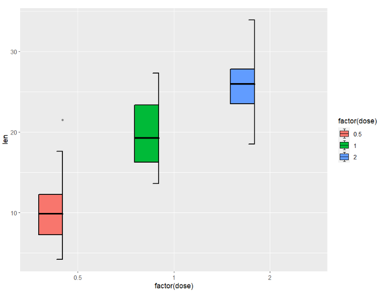
right type:
ggplot(ToothGrowth,aes(x = factor(dose),y = len)) +
  geom_jjboxplot(aes(fill = factor(dose)),
                 type = 'right')
we can use shift to ajust the position:
ggplot(ToothGrowth,aes(x = factor(dose),y = len)) +
  geom_jjboxplot(aes(fill = factor(dose)),
                 type = 'right',
                 shift = 0.05)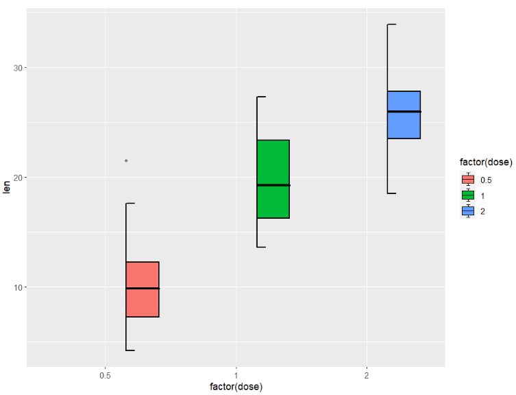
split type:
ggplot(ToothGrowth,aes(x = factor(dose),y = len)) +
  geom_jjboxplot(aes(fill = factor(dose)),
                 type = 'split')
in fact every boxplot includes two parts, you can also use shift to split them:
ggplot(ToothGrowth,aes(x = factor(dose),y = len)) +
  geom_jjboxplot(aes(fill = factor(dose)),
                 type = 'split',
                 split.shift = 0.025)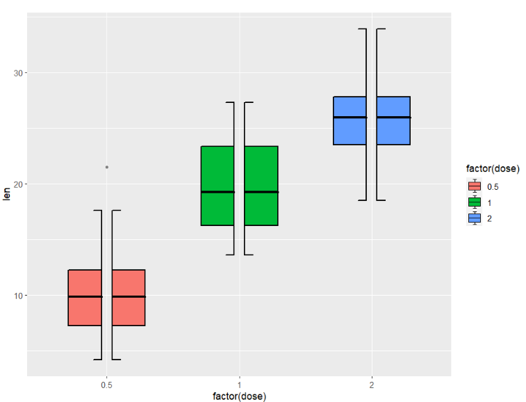
you can combine with other geom layer:
ggplot(ToothGrowth,aes(x = factor(dose),y = len)) +
  geom_jjboxplot(aes(fill = factor(dose)),
                 type = 'split',
                 split.shift = 0.08) +
  geom_violin(width = 0.15)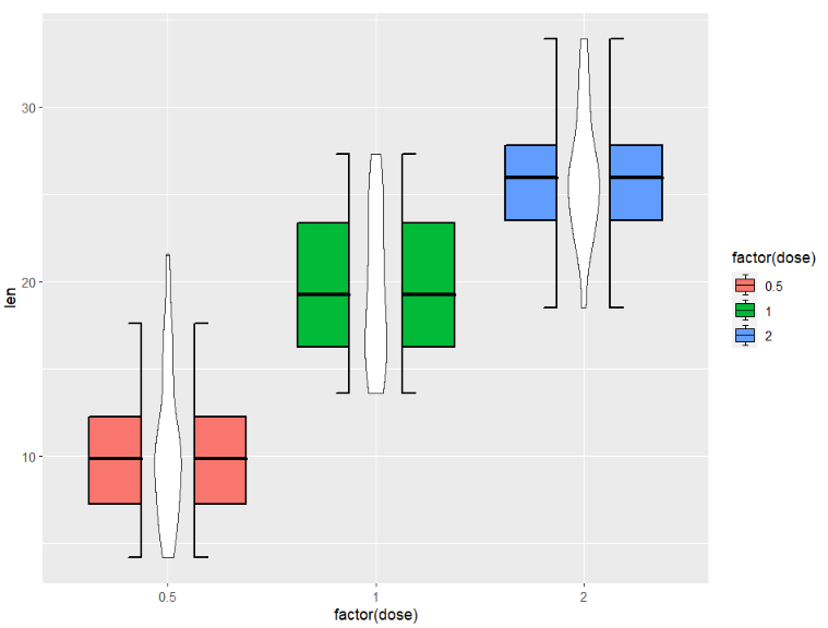
3.3 mached legend
you can add mached legend to split boxplot:
ggplot(ToothGrowth,aes(x = factor(dose),y = len)) +
  geom_jjboxplot(aes(fill = factor(dose)),
                 type = 'left',
                 key_glyph = draw_key_boxLeft)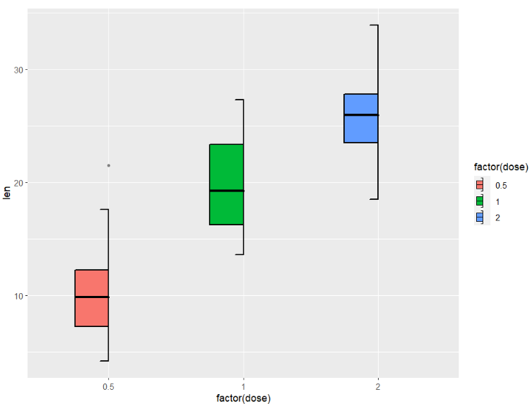
right:
ggplot(ToothGrowth,aes(x = factor(dose),y = len)) +
  geom_jjboxplot(aes(fill = factor(dose)),
                 type = 'right',
                 key_glyph = draw_key_boxRight)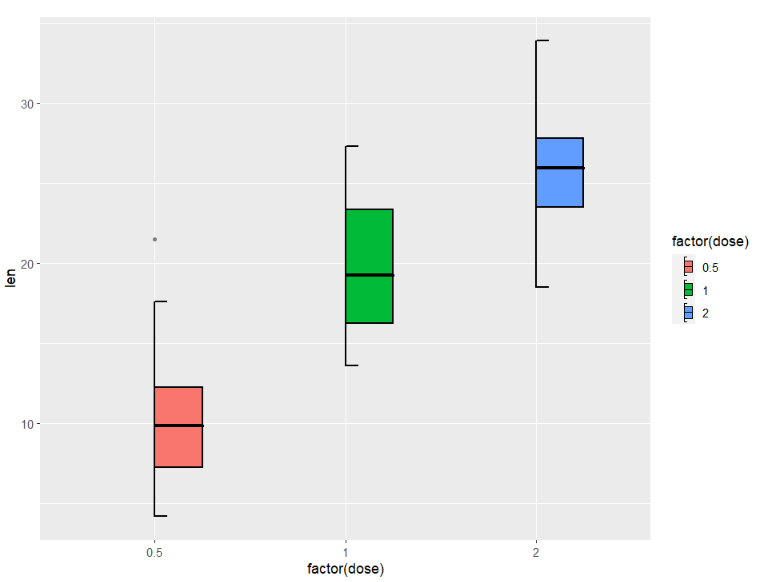
split:
ggplot(ToothGrowth,aes(x = factor(dose),y = len)) +
  geom_jjboxplot(aes(fill = factor(dose)),
                 type = 'split',
                 split.shift = 0.025,
                 key_glyph = draw_key_boxSplit)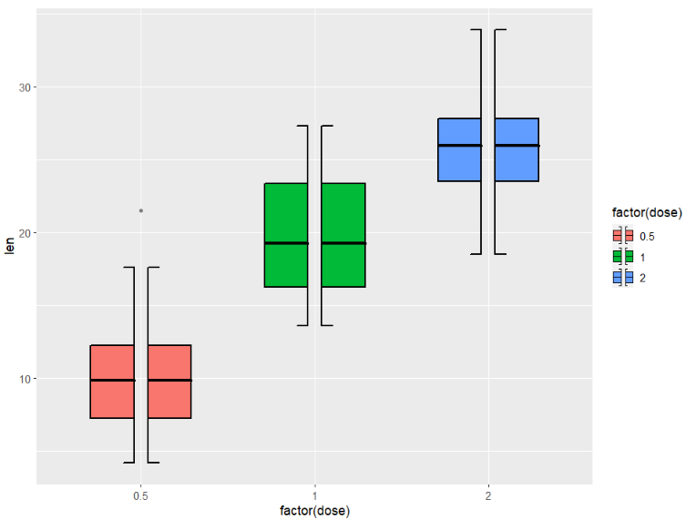
3.4 mapping with type
you can also define the type args as a mapping variable to draw different directions graphs especially for two sub-groups within group.
here we add a two types column into dataset:
# add type
ToothGrowth$type <- ifelse(ToothGrowth$supp == "OJ","left","right")
mapping with type:
ggplot(ToothGrowth,aes(x = factor(dose),y = len)) +
  geom_jjboxplot(aes(fill = supp,type = type),
                 width = 0.7)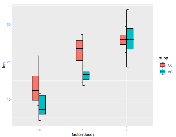
ajust group space:
ggplot(ToothGrowth,aes(x = factor(dose),y = len)) +
  geom_jjboxplot(aes(fill = supp,type = type),
                 width = 0.7,
                 position = position_dodge(width = 0.2))