Chapter 4 geom_jjviolin
I also re-write the geom_violin based on my knowledge and I also add more parameters to control the graphs to be plot. The following shows the details.
4.1 basic plot
we can show the difference between the geom_jjviolin and geom_violin:
p1 <-
  ggplot(mtcars,aes(x = factor(cyl),y = mpg)) +
  geom_violin()

p2 <-
  ggplot(mtcars,aes(x = factor(cyl),y = mpg)) +
  geom_jjviolin(width = 0.5)

cowplot::plot_grid(p1,p2,align = 'hv')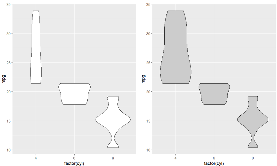
it seems that my violins are fatter than geom_violin’S?
we can also retain head and tail:
pt1 <-
  ggplot(mtcars,aes(x = factor(cyl),y = mpg)) +
  geom_violin(trim = F)

pt2 <-
  ggplot(mtcars,aes(x = factor(cyl),y = mpg)) +
  geom_jjviolin(width = 0.5,
                trim = F)

cowplot::plot_grid(pt1,pt2,align = 'hv')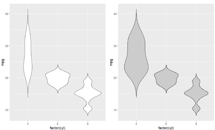
you can change the width:
ggplot(mtcars,aes(x = factor(cyl),y = mpg)) +
  geom_jjviolin(aes(fill = factor(cyl)),
                width = 0.2)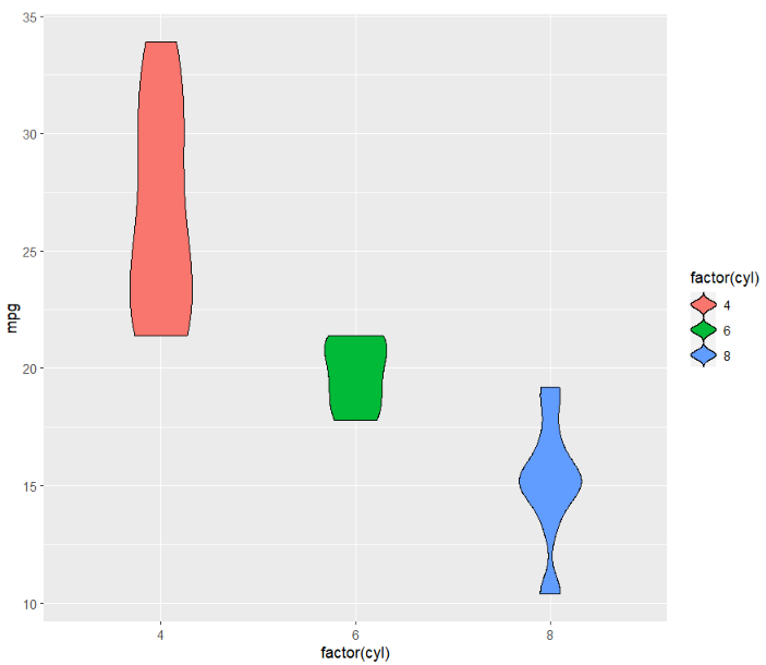
4.2 split violin
I supply four types to show the boxplot including full, split, left and right which can make violin plot more flexible for you.
full type(default mode):
ggplot(mtcars,aes(x = factor(cyl),y = mpg)) +
  geom_jjviolin(aes(fill = factor(cyl)),
                width = 0.5,
                trim = F,
                type = 'full')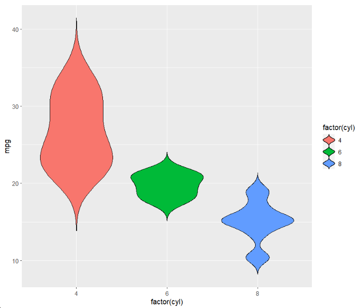
left type:
ggplot(mtcars,aes(x = factor(cyl),y = mpg)) +
  geom_jjviolin(aes(fill = factor(cyl)),
                width = 0.5,
                trim = F,
                type = 'left')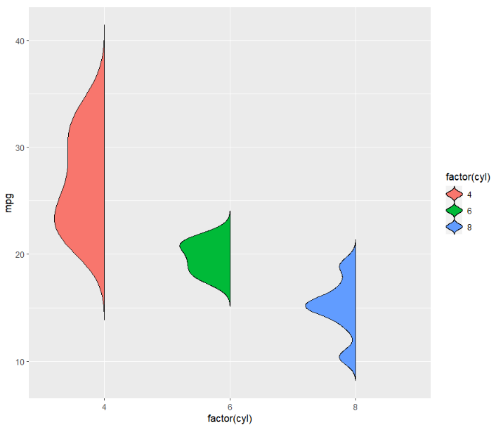
we can use shift to ajust the position:
ggplot(mtcars,aes(x = factor(cyl),y = mpg)) +
  geom_jjviolin(aes(fill = factor(cyl)),
                width = 0.5,
                trim = F,
                type = 'left',
                shift = 0.05)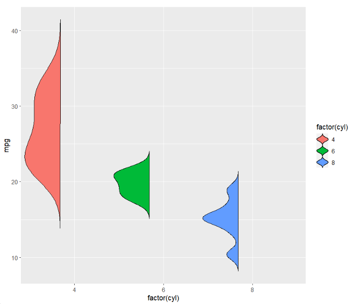
right type:
ggplot(mtcars,aes(x = factor(cyl),y = mpg)) +
  geom_jjviolin(aes(fill = factor(cyl)),
                width = 0.5,
                trim = F,
                type = 'right')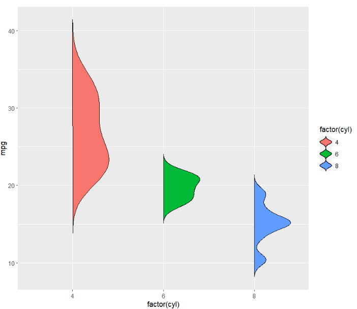
we can use shift to ajust the position:
ggplot(mtcars,aes(x = factor(cyl),y = mpg)) +
  geom_jjviolin(aes(fill = factor(cyl)),
                width = 0.5,
                trim = F,
                type = 'right',
                shift = 0.05)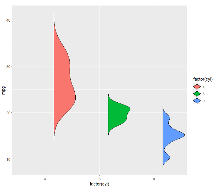
split type:
ggplot(mtcars,aes(x = factor(cyl),y = mpg)) +
  geom_jjviolin(aes(fill = factor(cyl)),
                width = 0.5,
                trim = F,
                type = 'split')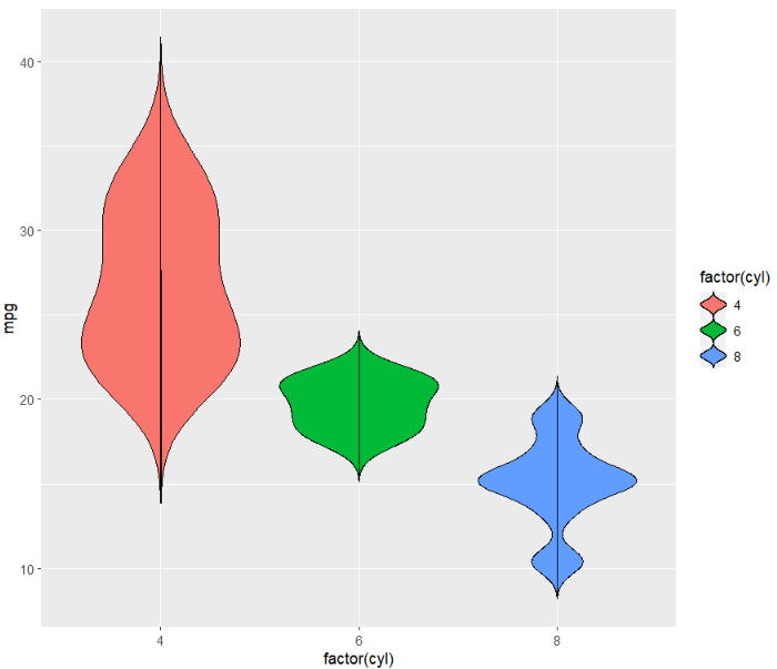
use split to split them:
ggplot(mtcars,aes(x = factor(cyl),y = mpg)) +
  geom_jjviolin(aes(fill = factor(cyl)),
                width = 0.5,
                trim = F,
                type = 'split',
                shift = 0.025)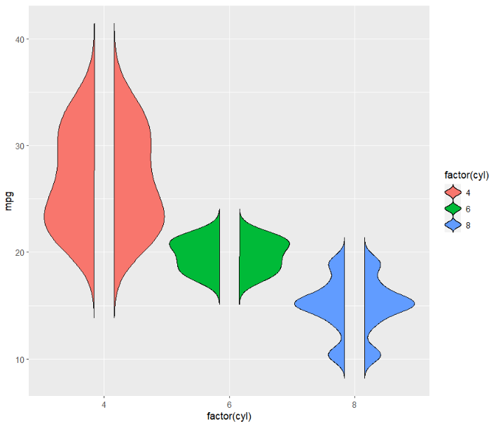
combine with other geom layer:
ggplot(mtcars,aes(x = factor(cyl),y = mpg)) +
  geom_jjviolin(aes(fill = factor(cyl)),
                width = 0.5,
                trim = F,
                type = 'split',
                shift = 0.025) +
  geom_boxplot(aes(fill = factor(cyl)),
               width = 0.1,alpha = 0.5)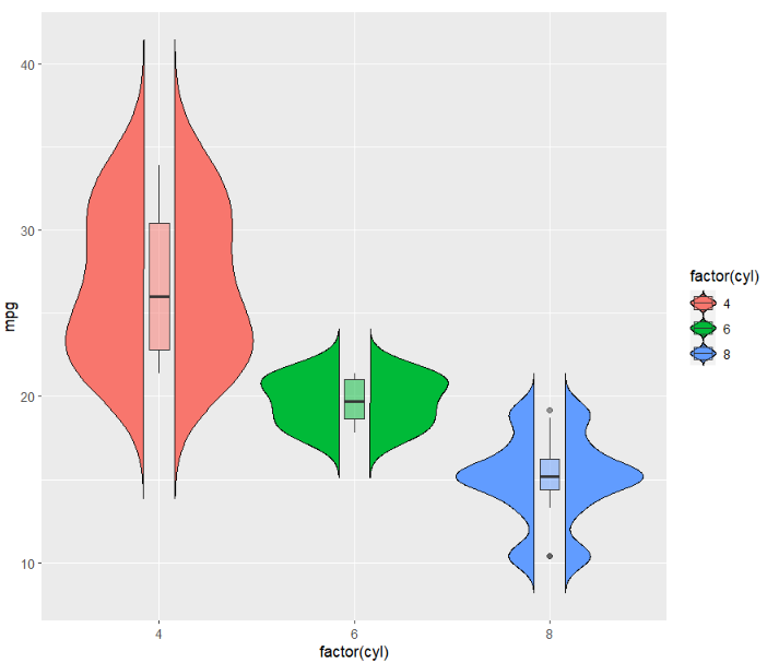
4.3 multiple groups
here we show geom_jjviolin works with multiple groups:
ggplot(ToothGrowth,aes(x = factor(dose),y = len)) +
  geom_jjviolin(aes(fill = supp),
                width = 0.25,
                trim = F,
                position = position_dodge(width = 1))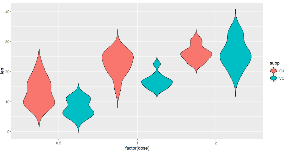
draw left:
ggplot(ToothGrowth,aes(x = factor(dose),y = len)) +
  geom_jjviolin(aes(fill = supp),
                width = 0.25,
                trim = F,
                position = position_dodge(width = 1),
                type = "left")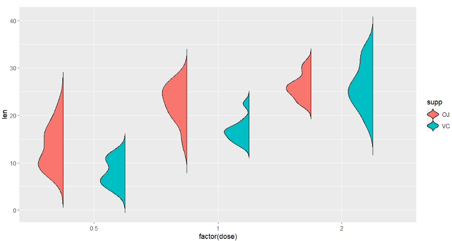
draw right:
ggplot(ToothGrowth,aes(x = factor(dose),y = len)) +
  geom_jjviolin(aes(fill = supp),
                width = 0.25,
                trim = F,
                position = position_dodge(width = 1),
                type = "right")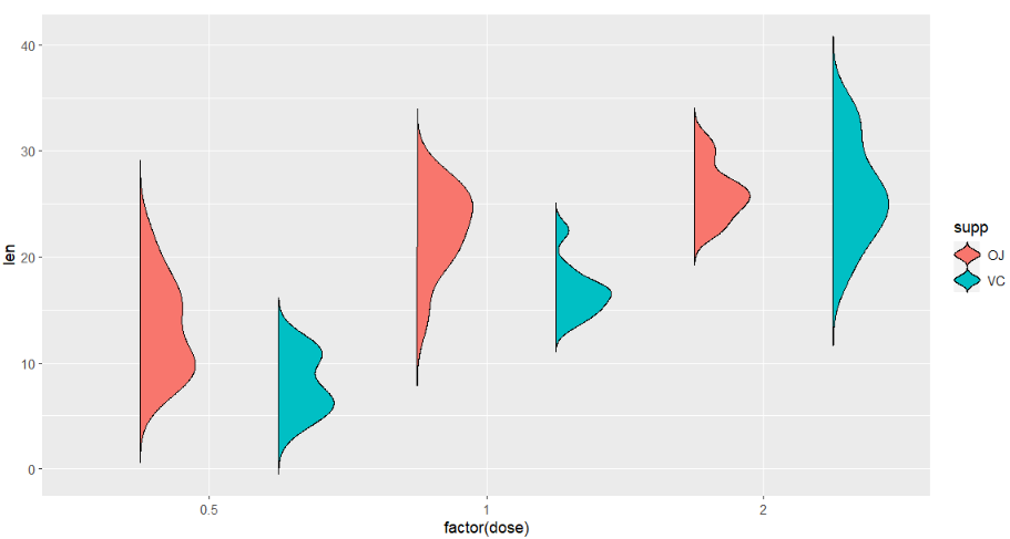
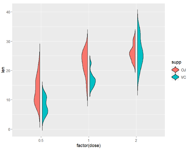
draw split:
ggplot(ToothGrowth,aes(x = factor(dose),y = len)) +
  geom_jjviolin(aes(fill = supp),
                width = 0.15,
                trim = F,
                position = position_dodge(width = 1),
                type = "split",
                shift = 0.03)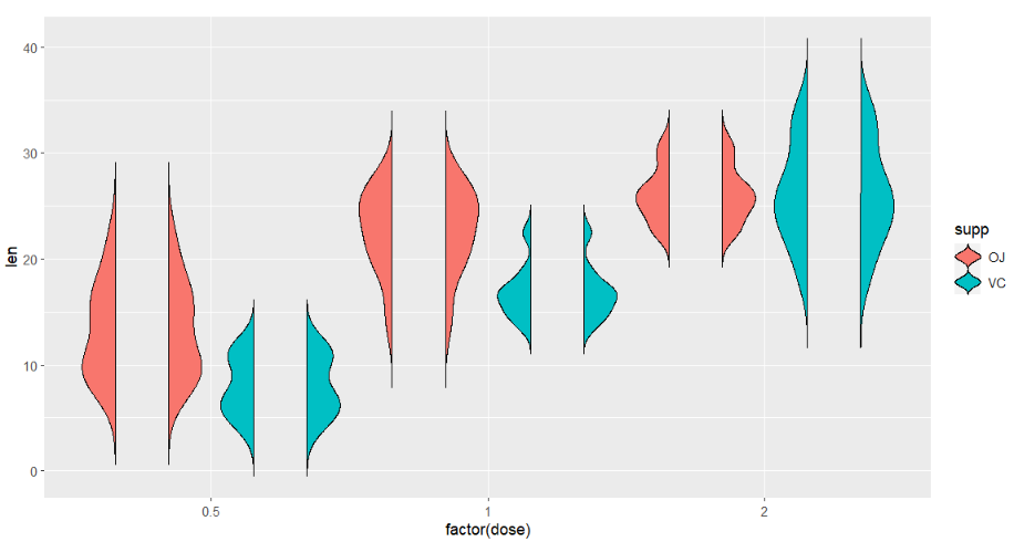
combine with other geom layer:
ggplot(ToothGrowth,aes(x = factor(dose),y = len)) +
  geom_jjviolin(aes(fill = supp),
                width = 0.15,
                trim = F,
                position = position_dodge(width = 1),
                type = "split",
                shift = 0.03,
                key_glyph = draw_key_violinSplit) +
  geom_boxplot(aes(fill = supp),
               width = 0.2,
               alpha = 0.5,
               position = position_dodge(width = 1))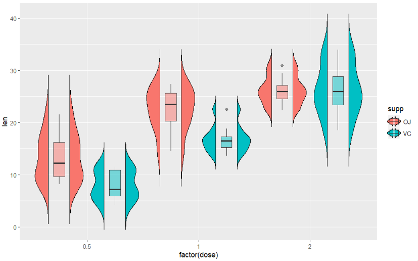
4.4 mached legend
you can add mached legend to split violin plot:
ggplot(mtcars,aes(x = factor(cyl),y = mpg)) +
  geom_jjviolin(aes(fill = factor(cyl)),
                width = 0.5,
                trim = F,
                type = 'left',
                key_glyph = draw_key_violinLeft)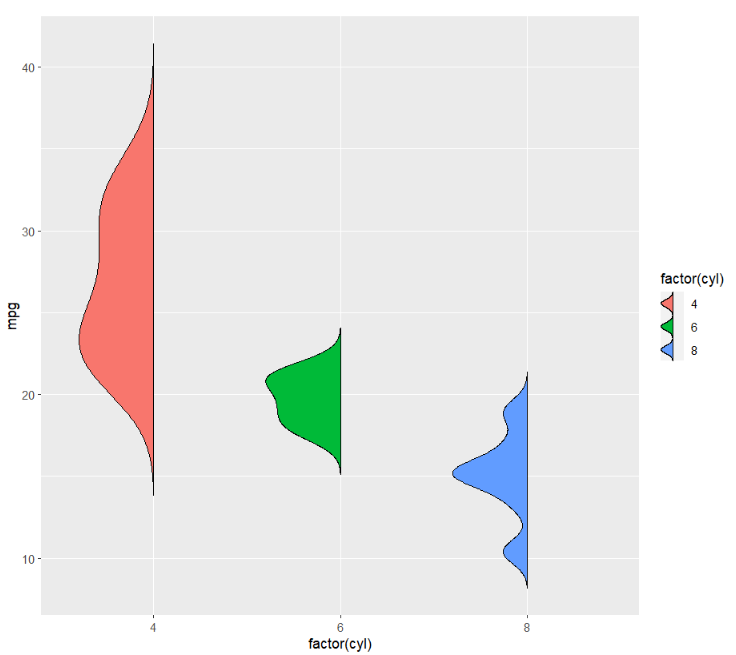
right legend:
ggplot(mtcars,aes(x = factor(cyl),y = mpg)) +
  geom_jjviolin(aes(fill = factor(cyl)),
                width = 0.5,
                trim = F,
                type = 'right',
                key_glyph = draw_key_violinRight)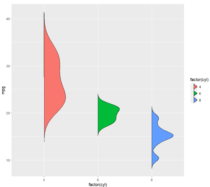
split legend:
ggplot(mtcars,aes(x = factor(cyl),y = mpg)) +
  geom_jjviolin(aes(fill = factor(cyl)),
                width = 0.5,
                trim = F,
                type = 'split',
                shift = 0.025,
                key_glyph = draw_key_violinSplit)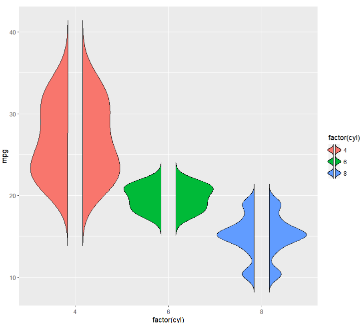
4.5 mapping with type
you can also define the type args as a mapping variable to draw different directions graphs especially for two sub-groups within group.
mapping with type:
# add type
ToothGrowth$type <- ifelse(ToothGrowth$supp == "OJ","left","right")

ggplot(ToothGrowth,aes(x = factor(dose),y = len)) +
  geom_jjviolin(aes(fill = supp,
                    type = type),
                width = 0.15,
                trim = F)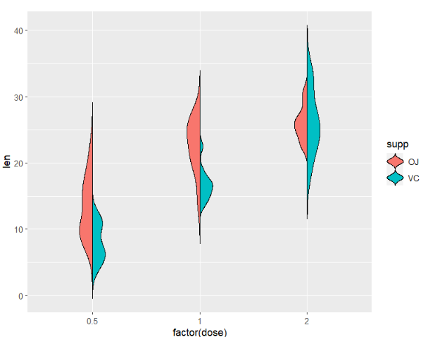
ajust group space:
ggplot(ToothGrowth,aes(x = factor(dose),y = len)) +
  geom_jjviolin(aes(fill = supp,
                    type = type),
                width = 0.15,
                trim = F,
                position = position_dodge(width = 0.1))