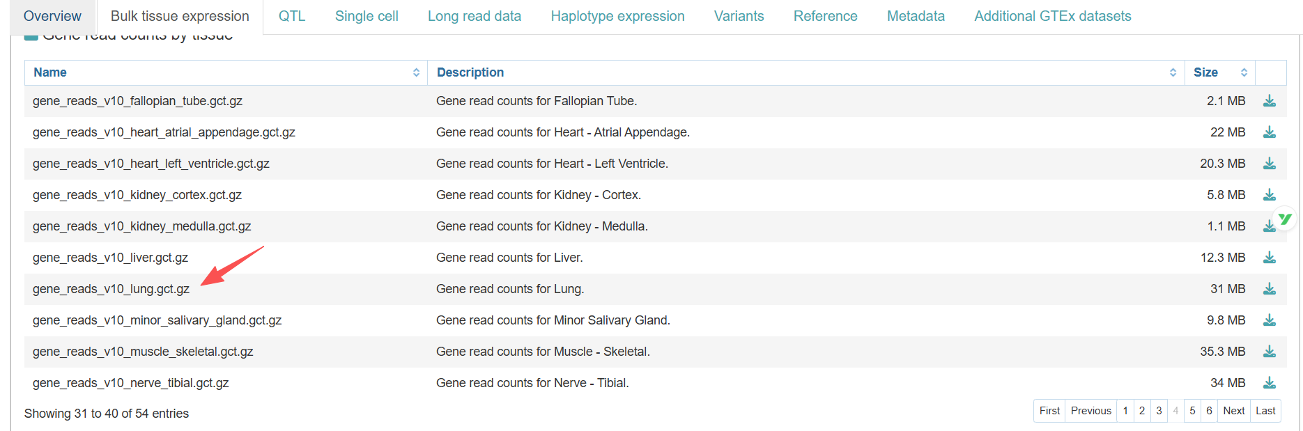
wget https://storage.googleapis.com/adult-gtex/bulk-gex/v10/rna-seq/counts-by-tissue/gene_reads_v10_lung.gct.gz4 Integration of GTEx normal tissue samples
4.1 Introduction
TCGA datasets typically contain abundant tumor samples but relatively limited matched normal tissue samples. The GTEx database (https://www.gtexportal.org/home/) provides extensive RNA-seq data from normal tissues across various organs. By integrating GTEx normal samples with TCGA tumor data, researchers can mitigate analytical biases arising from insufficient normal controls. OMICSCOPE facilitates this integration by directly incorporating user-downloaded GTEx count data, streamlining the analytical workflow.
4.2 GTEx read counts download
Here, we downloaded normal lung tissue count data from the GTEx database, as TCGA-LUAD contains only 59 normal samples, which is relatively limited:
4.3 Object construction
We then build the omicscope object by providing the downloaded GTEx count data to the gtex_counts_data parameter:
obj <- ucscZenaToObj(gtf_anno = "gencode.v36.annotation.gtf.gz",
                     counts_data = "TCGA-LUAD.star_counts.tsv.gz",
                     pheno_data = "TCGA-LUAD.clinical.tsv.gz",
                     survival_data = "TCGA-LUAD.survival.tsv.gz",
                     gtex_counts_data = "gene_reads_v10_lung.gct.gz")

obj
# class: omicscope
# dim: 52739 1193
# metadata(0):
# assays(1): counts
# rownames(52739): ENSG00000223972.5 ENSG00000227232.5 ... ENSG00000210195.2 ENSG00000210196.2
# rowData names(3): gene_id gene_name gene_biotype
# colnames(1193): TCGA-38-7271-01A TCGA-55-7914-01A ... GTEX-ZZPT-1326-SM-5E43H GTEX-ZZPU-0526-SM-5E44U
# colData names(97): sample id ... X_PATIENT group2
4.4 Data normalization and reduction
The next critical step is to examine whether batch effects exist between the GTEx normal tissue samples and TCGA normal samples. If batch effects are present and left uncorrected, they may confound results and lead to erroneous conclusions in downstream analyses:
obj <- normalize_data(obj, norm_type = "tpm")

obj <- run_reduction(object = obj,
                     reduction = "pca",
                     top_hvg_genes = 3000)

obj <- run_reduction(object = obj,
                     reduction = "umap",
                     top_hvg_genes = 3000)

obj <- run_reduction(object = obj,
                     reduction = "tsne",
                     top_hvg_genes = 3000)

p1 <- dim_plot(obj, reduction = "pca", color_by = "group2")
p2 <- dim_plot(obj, reduction = "umap", color_by = "group2")
p3 <- dim_plot(obj, reduction = "tsne", color_by = "group2")


cowplot::plot_grid(plotlist = list(p1,p2,p3),
                   ncol = 2)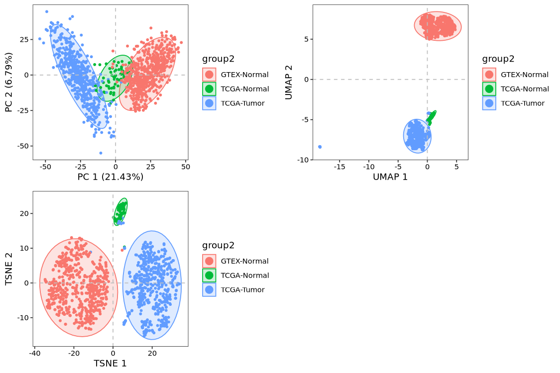
Visualizations from all three dimensionality reduction approaches consistently reveal pronounced batch effects, with GTEx samples clearly segregating from patient-derived normal tissue samples.
4.5 Batch effect removal
To address the observed batch effects, we employ the ComBat-seq method through the correct_batch_effect function. Note that batch correction will replace the original count matrix with adjusted values. After applying this correction, we perform dimensionality reduction analyses again to assess whether samples now cluster by biological characteristics rather than technical batch:
obj <- correct_batch_effect(obj)
# Found 2 batches
# Using full model in ComBat-seq.
# Adjusting for 1 covariate(s) or covariate level(s)
# Estimating dispersions
# Fitting the GLM model
# Shrinkage off - using GLM estimates for parameters
# Adjusting the data

obj <- normalize_data(obj, norm_type = "tpm")

obj <- run_reduction(object = obj,
                     reduction = "pca",
                     top_hvg_genes = 3000)

obj <- run_reduction(object = obj,
                     reduction = "umap",
                     top_hvg_genes = 3000)

obj <- run_reduction(object = obj,
                     reduction = "tsne",
                     top_hvg_genes = 3000)

p1 <- dim_plot(obj, reduction = "pca", color_by = "group2")
p2 <- dim_plot(obj, reduction = "umap", color_by = "group2")
p3 <- dim_plot(obj, reduction = "tsne", color_by = "group2")


cowplot::plot_grid(plotlist = list(p1,p2,p3),
                   ncol = 2)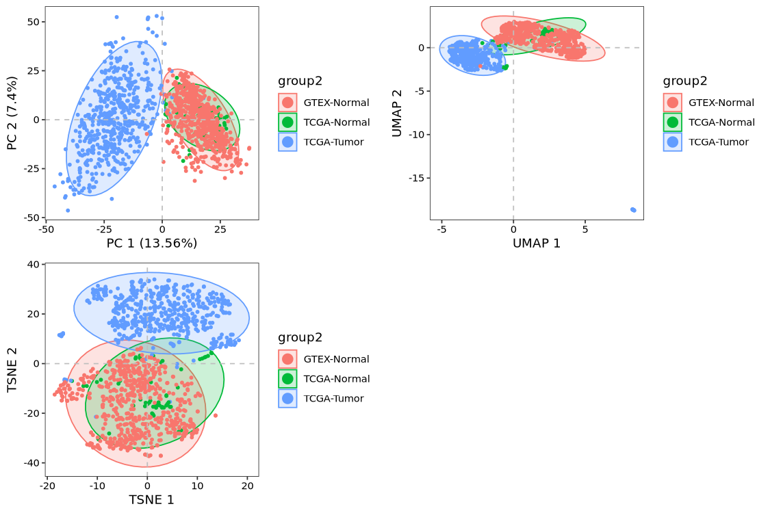
With batch effects successfully corrected, users can now proceed with standard downstream analyses, including differential expression, pathway enrichment, and other routine procedures.