5  Integration of TCGAbiolinks

5.1 Introduction

omicScope is now compatible with TCGAbiolinks-curated gene expression matrices stored as SummarizedExperiment objects. Future development will extend compatibility to other data types.

5.2 Retrieving gene expression data with TCGAbiolinks

For demonstration purposes, we’ll download the expression matrix for LUAD (lung adenocarcinoma) using TCGAbiolinks. The following sample code returns a SummarizedExperiment object:

# BiocManager::install("TCGAbiolinks")
library(TCGAbiolinks)
library(SummarizedExperiment)

query.exp <- GDCquery(
  project = "TCGA-LUAD",
  data.category = "Transcriptome Profiling",
  data.type = "Gene Expression Quantification",
  workflow.type = "STAR - Counts"
)

GDCdownload(
  query = query.exp,
  files.per.chunk = 200
)

luad.exp <- GDCprepare(
  query = query.exp,
  save = TRUE,
  save.filename = "luadExp.rda"
)

5.3 omicscope object construction

The TCGAbiolinksToObj function facilitates the conversion of SummarizedExperiment objects from TCGAbiolinks into omicScope objects. To enhance your analysis, we’ve included the gtex_counts_data parameter, which allows you to integrate counts data from corresponding normal tissues in the GTEx database:

library(omicScope)

load("luadExp.rda")

# obj <- TCGAbiolinksToObj(tcgabiolinks_obj = data)

obj <- TCGAbiolinksToObj(gtf_anno = "gencode.v36.annotation.gtf.gz",
                         tcgabiolinks_obj = data,
                         gtex_counts_data = "gene_reads_v10_lung.gct.gz")
obj
# class: omicscope 
# dim: 52739 1204 
# metadata(0):
# assays(1): counts
# rownames(52739): ENSG00000223972.5 ENSG00000227232.5 ... ENSG00000210195.2 ENSG00000210196.2
# rowData names(3): gene_id gene_name gene_biotype
# colnames(1204): TCGA-44-6147-01B-06R-A277-07 TCGA-44-6147-01A-11R-1755-07 ...
#   GTEX-ZZPT-1326-SM-5E43H GTEX-ZZPU-0526-SM-5E44U
# colData names(99): sample patient ... OS group2

5.4 Downstream analysis

Now that we have our omicscope object, we’re ready to perform downstream analyses! This includes quality control checks, batch effect correction, differential expression analysis, and other analytical steps:

obj <- normalize_data(obj)

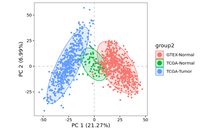
obj <- run_reduction(obj, top_hvg_genes = 3000)

dim_plot(obj, color_by = "group2")