Chapter 5 Basic visualization
There are multiple chapters to illustrate how to use trackVisProMax draw basic tracks.
Raw fastqs can be fetched CRA003985, You need download them and map to genome and convert bam files to bigwig format.
First we load test data into R:
library(ggplot2)
library(BioSeqUtils)

# load bigwig files
file <- list.files(path = "test-bw/",pattern = '.bw',full.names = T)
file
# [1] "test-bw/1cell-m6A-1.bw" "test-bw/1cell-m6A-2.bw" "test-bw/1cell-RNA-1.bw"
# [4] "test-bw/1cell-RNA-2.bw" "test-bw/2cell-m6A-1.bw" "test-bw/2cell-m6A-2.bw"
# [7] "test-bw/2cell-RNA-1.bw" "test-bw/2cell-RNA-2.bw"

# select some chromosomes for test
bw <- loadBigWig(file,chrom = c("5","15"))

# check
head(bw,3)
#   seqnames   start     end   score    fileName
# 1       15       1 3054635 0.00000 1cell-m6A-1
# 2       15 3054636 3054640 1.34079 1cell-m6A-1
# 3       15 3054641 3054715 2.68159 1cell-m6A-1

# gtf
gtf <- rtracklayer::import.gff("Mus_musculus.GRCm38.102.gtf",format = "gtf") %>%
  data.frame()
5.1 Basic plot
Plot with given one gene symbol (make sure the gene_name column in your annotation file):
Plot multiple genes at the same time:
 Change track colors with color vectors:
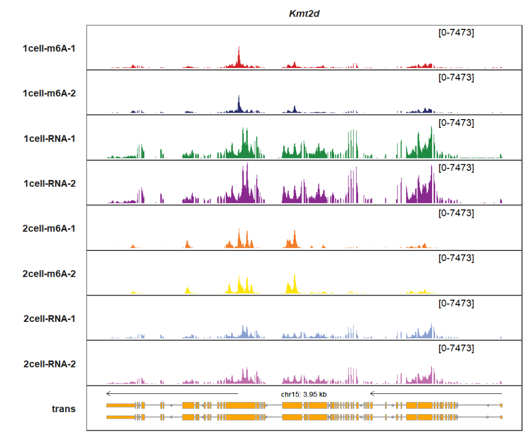
trackVisProMax(Input_gtf = gtf,
               Input_bw = bw,
               Input_gene = c("Kmt2d"),
               sample_fill_col = c(rep(c("red","red","grey50","grey50"),3)))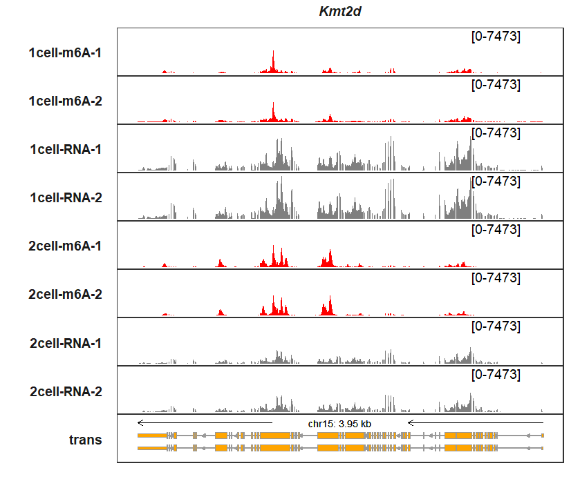
Or you can give a named vector to assign colors for each track:
trmycol <- c("1cell-m6A-1" = "orange", "1cell-m6A-2" = "orange",
           "1cell-RNA-1" = "green", "1cell-RNA-2"  = "green",
           "2cell-m6A-1" = "blue", "2cell-m6A-2" = "blue",
           "2cell-RNA-1" = "pink", "2cell-RNA-2" = "pink")

trackVisProMax(Input_gtf = gtf,
               Input_bw = bw,
               Input_gene = c("Kmt2d"),
               sample_fill_col = mycol)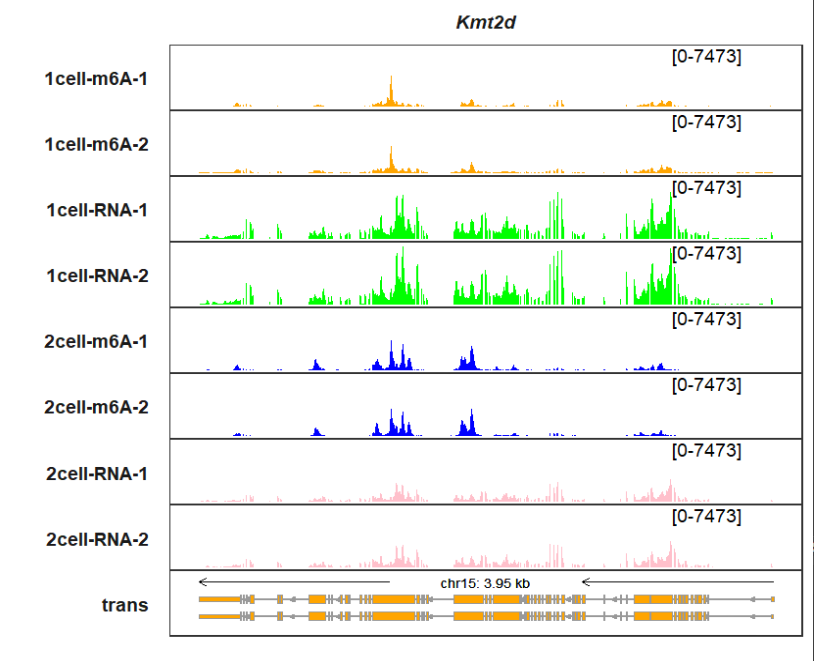
Adding genomic region label:
trackVisProMax(Input_gtf = gtf,
               Input_bw = bw,
               Input_gene = c("Kmt2d","Dnaaf5","Zfp68"),
               add_gene_region_label = T)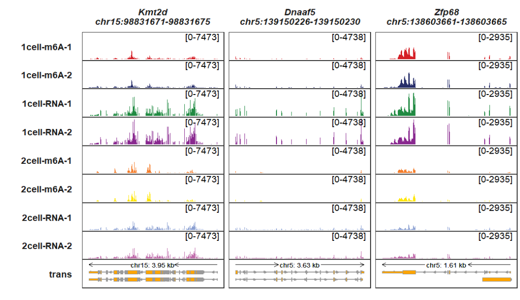
Adding legend:
trackVisProMax(Input_gtf = gtf,
               Input_bw = bw,
               Input_gene = c("Kmt2d","Dnaaf5","Zfp68"),
               add_gene_region_label = T,
               signal_layer_bw_params = list(show.legend = T))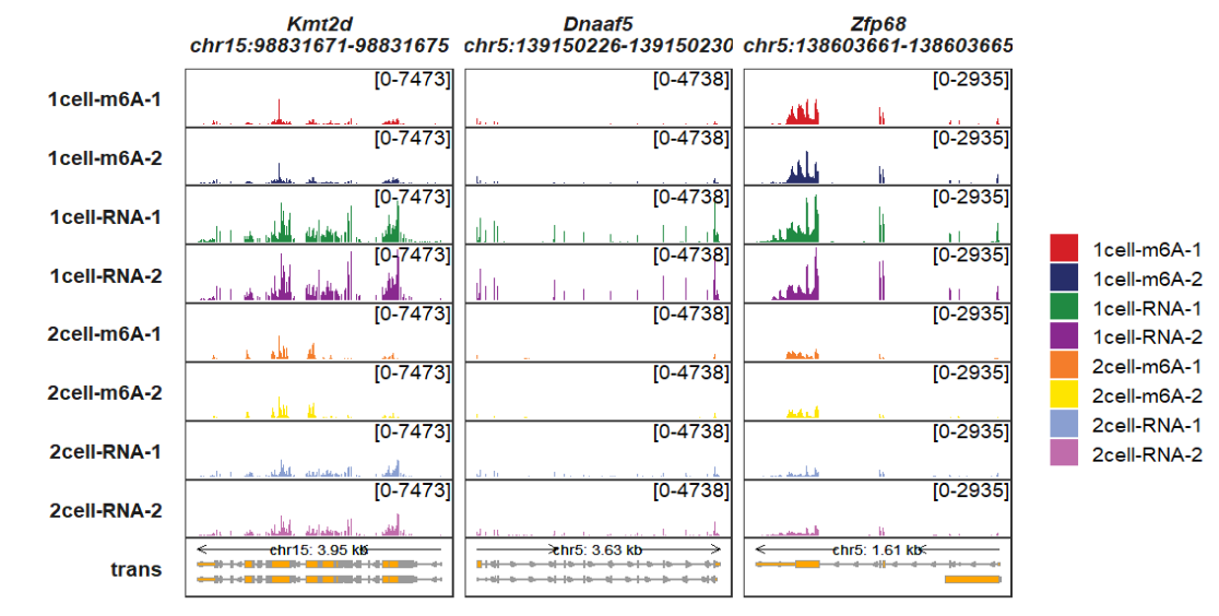
5.2 Signal range settings
signal_range_pos can be used to change the y axis limitation range label position:
trackVisProMax(Input_gtf = gtf,
               Input_bw = bw,
               Input_gene = c("Kmt2d","Dnaaf5"),
               signal_range_pos = c(0.1,0.85))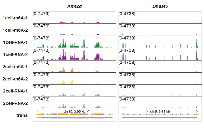
signal_range_label_params can be used to change the y label styles:
trackVisProMax(Input_gtf = gtf,
               Input_bw = bw,
               Input_gene = c("Kmt2d","Dnaaf5"),
               signal_range_pos = c(0.1,0.85),
               signal_range_label_params = list(size = 2,color = "red"))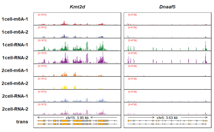
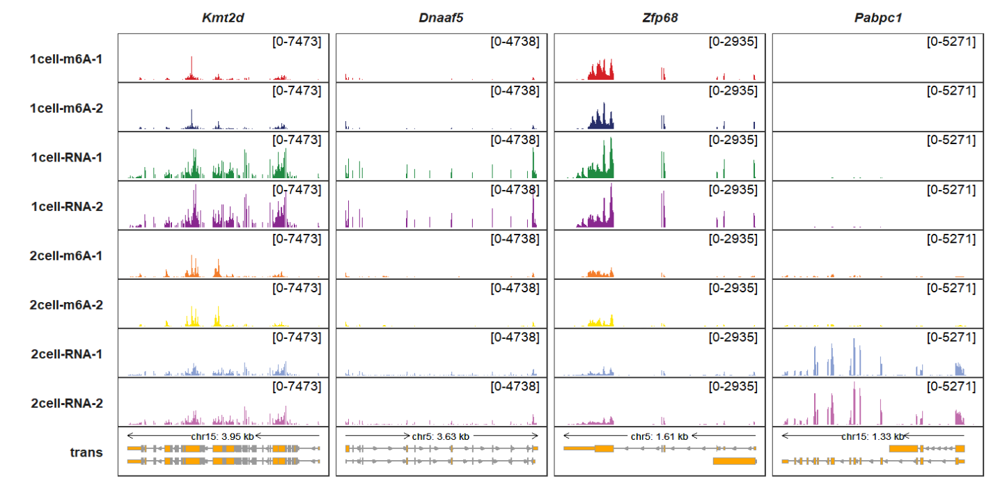
As you can see, the signal range is same by each column panel, you can set fixed_column_range = F to make free scales for each panel:
trackVisProMax(Input_gtf = gtf,
               Input_bw = bw,
               Input_gene = c("Kmt2d","Dnaaf5","Zfp68","Pabpc1"),
               fixed_column_range = F)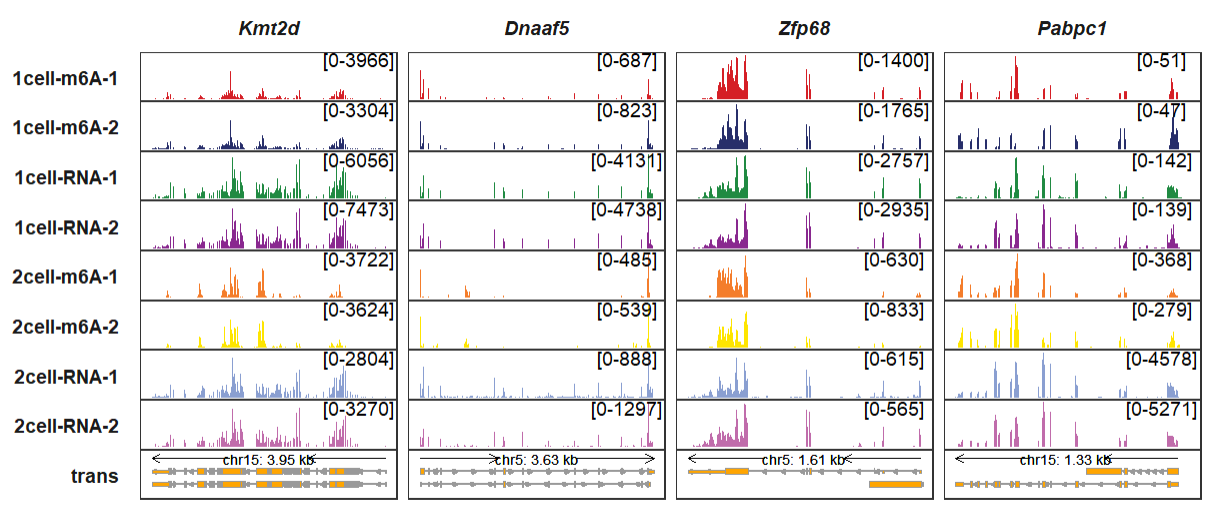
Giving a named list with named vectors to control signal range for each panel:
sample <- c("1cell-m6A-1","1cell-m6A-2","1cell-RNA-1","1cell-RNA-2",
"2cell-m6A-1","2cell-m6A-2","2cell-RNA-1","2cell-RNA-2")
Kmt2d_rg <- c(rep(4000,2),rep(8000,2),rep(4000,4))
names(Kmt2d_rg) <- sample
Kmt2d_rg
# 1cell-m6A-1 1cell-m6A-2 1cell-RNA-1 1cell-RNA-2 2cell-m6A-1 2cell-m6A-2 2cell-RNA-1 2cell-RNA-2
# 4000 4000 8000 8000 4000 4000 4000 4000
Dnaaf5_rg <- c(rep(1000,2),rep(5000,2),rep(2000,4))
names(Dnaaf5_rg) <- sample
Dnaaf5_rg
# 1cell-m6A-1 1cell-m6A-2 1cell-RNA-1 1cell-RNA-2 2cell-m6A-1 2cell-m6A-2 2cell-RNA-1 2cell-RNA-2
# 1000 1000 5000 5000 2000 2000 2000 2000
trackVisProMax(Input_gtf = gtf,
Input_bw = bw,
Input_gene = c("Kmt2d","Dnaaf5"),
signal_range = list(Kmt2d = Kmt2d_rg,
Dnaaf5 = Dnaaf5_rg))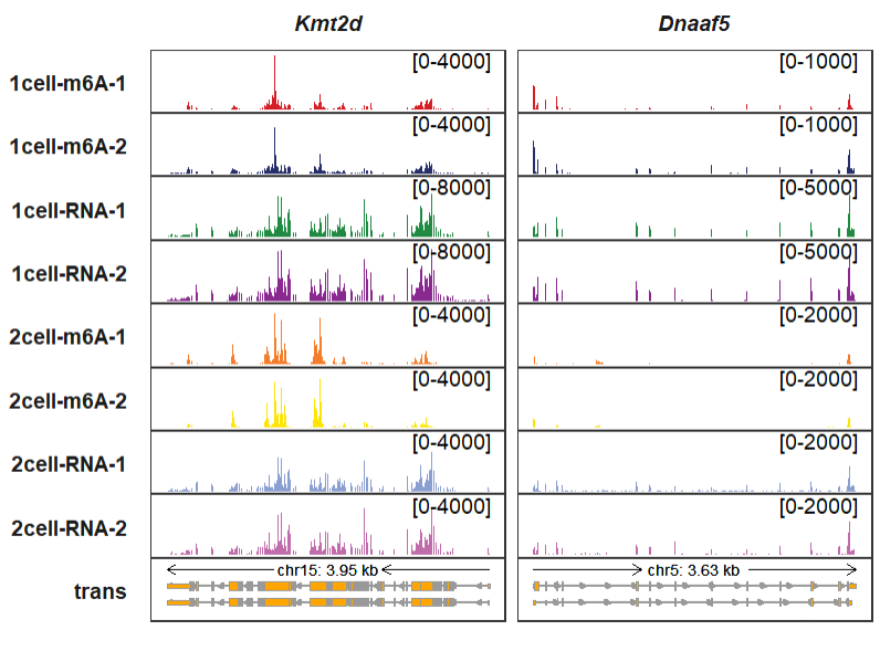 You can even set a range for a specified panel:
trackVisProMax(Input_gtf = gtf,
               Input_bw = bw,
               Input_gene = c("Kmt2d","Dnaaf5"),
               signal_range = list(Kmt2d = c("1cell-m6A-1" = 8000),
                                   Dnaaf5 = c("1cell-m6A-1" = 1000)))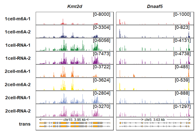
Containing negative values in signal file is also supported. Here we set the score range in (-500,500) and plot:
# load bigwig files
file <- list.files(path = "test-bw/",pattern = '.bw',full.names = T)[1:4]
file
# [1] "test-bw/1cell-m6A-1.bw" "test-bw/1cell-m6A-2.bw"
# "test-bw/1cell-RNA-1.bw" "test-bw/1cell-RNA-2.bw"
# select some chromosomes for test
bw <- loadBigWig(file,chrom = c("5","15"))
bw$score <- sample(seq(-500,500,0.5),size = nrow(bw),replace = T)
# gtf
gtf <- rtracklayer::import.gff("Mus_musculus.GRCm38.102.gtf",format = "gtf") %>%
data.frame()
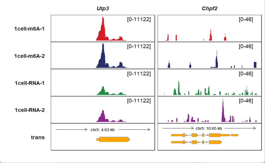
trackVisProMax(Input_gtf = gtf,
Input_bw = bw,
Input_gene = c("Utp3","Chpf2"))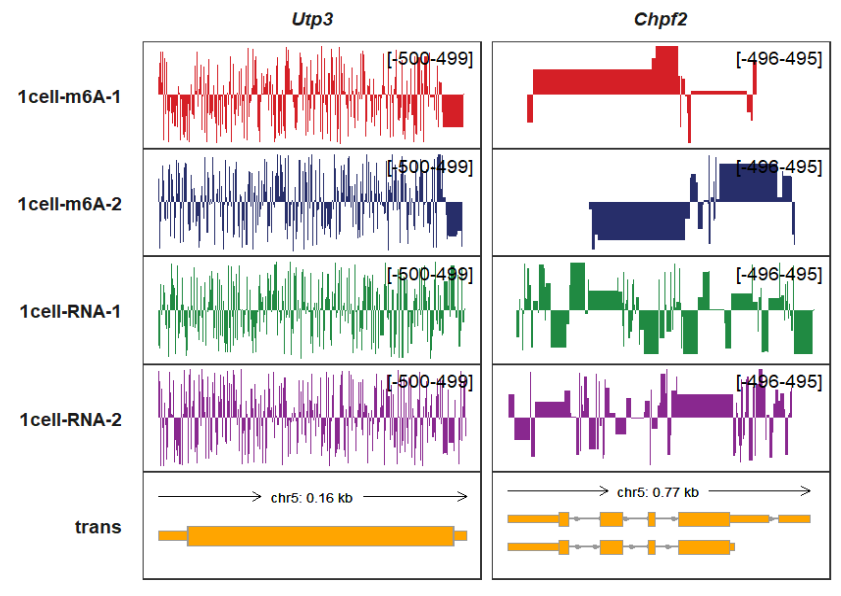 If you want to control the minimum value and maximum value for each panel, you can
give a named list with 2 element vectors in a named list for signal_range
parameter, here we show an example:
If you want to control the minimum value and maximum value for each panel, you can
give a named list with 2 element vectors in a named list for signal_range
parameter, here we show an example:
trackVisProMax(Input_gtf = gtf,
               Input_bw = bw,
               signal_range = list(Utp3 = list("1cell-m6A-1" = c(-1000,1000),
                                               "1cell-m6A-2" = c(0,1000),
                                               "1cell-RNA-1" = c(-1000,1000),
                                               "1cell-RNA-2" = c(-1000,0)),
                                   Chpf2 = c("1cell-m6A-1" = 1000,
                                             "1cell-RNA-2" = 500)),
               Input_gene = c("Utp3","Chpf2"))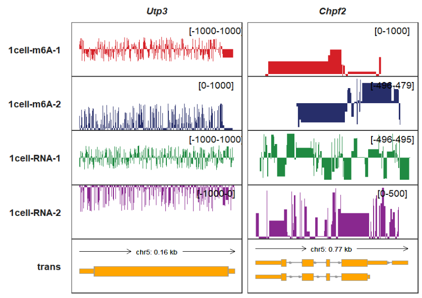
The genomic coordinate region id has been your gene mark to change the range for each panel:
trackVisProMax(Input_gtf = gtf,
               Input_bw = bw,
               query_region = list(query_chr = c("5","15"),
                                   query_start = c(65438603,9263295),
                                   query_end = c(65834288,9785835)),
               signal_range = list("chr5:65438603-65834288" =
                                     c("1cell-m6A-1" = 4000,"1cell-m6A-2" = 3000,
"1cell-RNA-1" = 2000,"1cell-RNA-2" = 1000))) 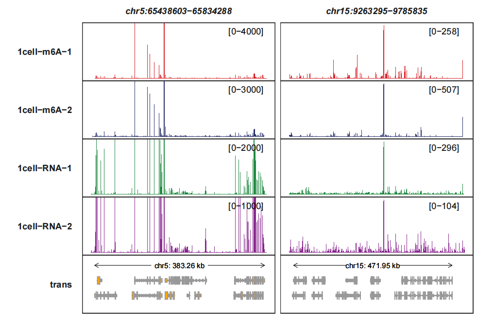
5.3 Transcript track settings
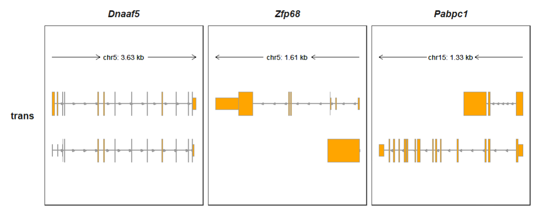
Here we illustrate some related parameters to draw the transcript track. trans_topN is used to control how many transcripts for a gene to be drawn in the track. The default is to show top 2 longest transcripts according to their transcipt exon length. You can change it with other values:
trackVisProMax(Input_gtf = gtf,
               Input_bw = bw,
               Input_gene = c("Dnaaf5","Zfp68","Pabpc1"),
               trans_topN = 1)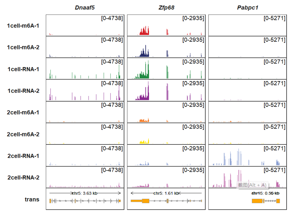
Showing top 5 transcripts:
trackVisProMax(Input_gtf = gtf,
               Input_bw = bw,
               Input_gene = c("Dnaaf5","Zfp68","Pabpc1"),
               trans_topN = 5)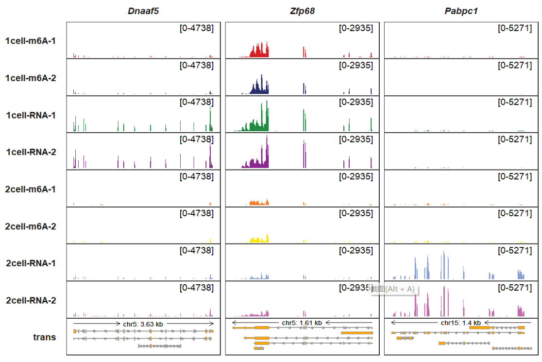
collapse_trans parameter allows you to collapse all transcripts you have shown in the trans track:
trackVisProMax(Input_gtf = gtf,
               Input_bw = bw,
               Input_gene = c("Dnaaf5","Zfp68","Pabpc1"),
               trans_topN = 5,
               collapse_trans = T)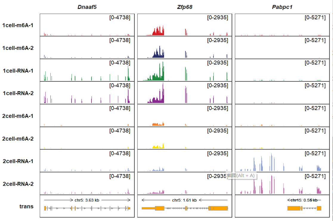
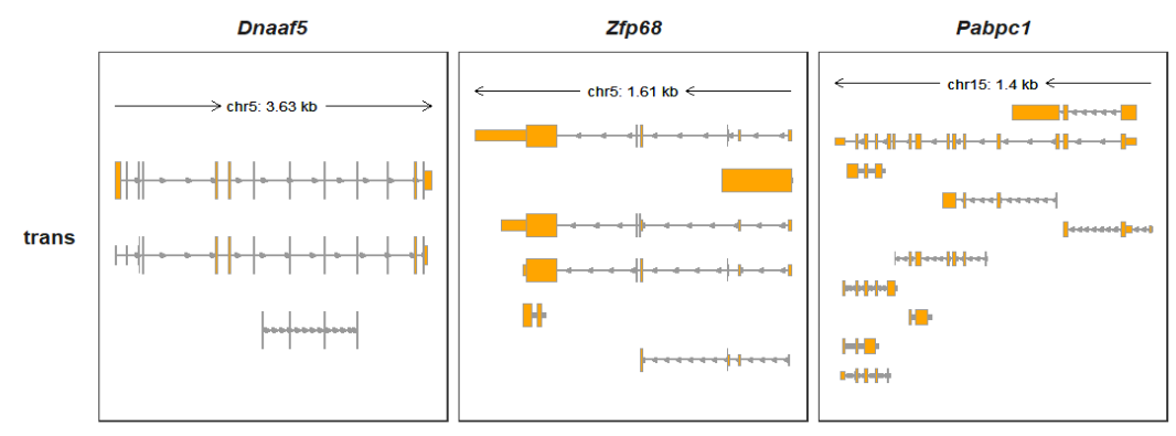
Setting trans_topN = “all” which can show all transcripts for a gene:
trackVisProMax(Input_gtf = gtf,
               Input_bw = bw,
               Input_gene = c("Dnaaf5","Zfp68","Pabpc1"),
               trans_topN = "all")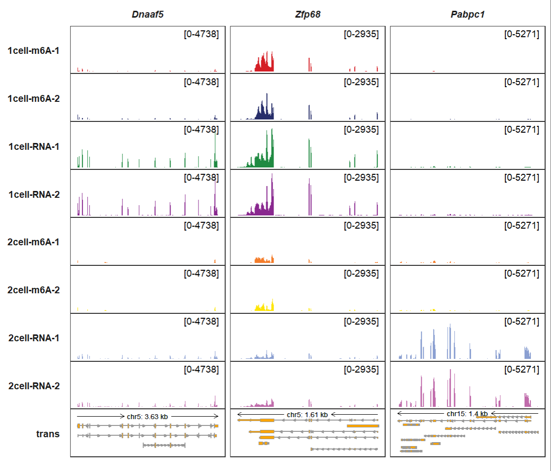
You can also collapse the transcripts:
trackVisProMax(Input_gtf = gtf,
               Input_bw = bw,
               Input_gene = c("Dnaaf5","Zfp68","Pabpc1"),
               trans_topN = "all",
               collapse_trans = T)
rel_len control the arrow densities on transcript, you can check createSegment function for details. arrow_rel_len_params_list accepts a list parameters to control how the arrows be generated. rel_len smaller, the more arrows be generated:
trackVisProMax(Input_gtf = gtf,
               Input_bw = bw,
               Input_gene = c("Actb","Myc","Mtdh"),
               arrow_rel_len_params_list = list(rel_len = 0.2))
More controls for arrows:
trackVisProMax(Input_gtf = gtf,
               Input_bw = bw,
               Input_gene = c("Actb","Myc","Mtdh"),
               arrow_rel_len_params_list = list(rel_len = 0.15),
               trans_exon_arrow_params = list(fill = "red",color = "red",
                                              linewidth = 1))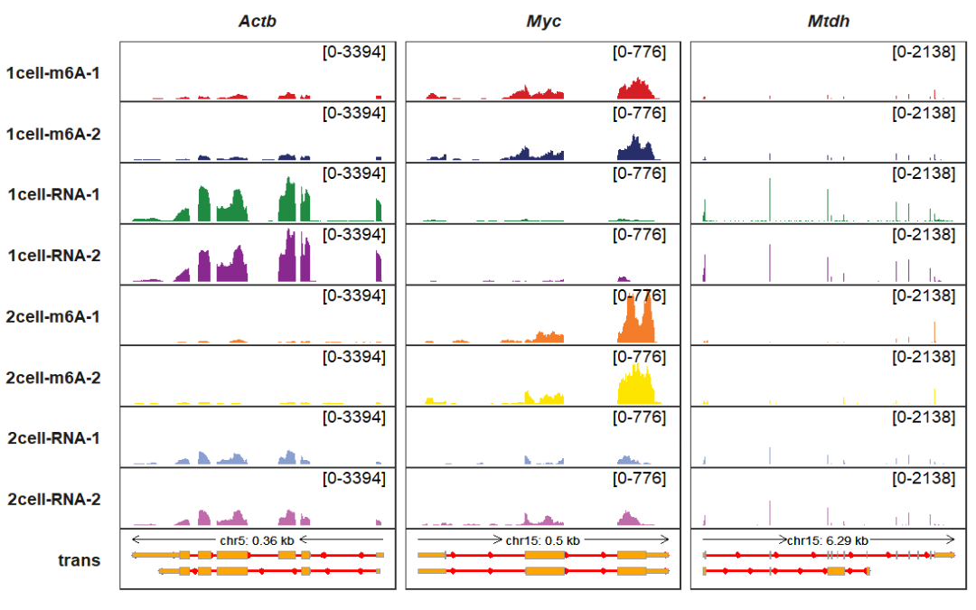
Changing arrow styles:
trackVisProMax(Input_gtf = gtf,
               Input_bw = bw,
               Input_gene = c("Actb","Myc","Mtdh"),
               arrow_rel_len_params_list = list(rel_len = 0.15),
               trans_exon_arrow_params = list(arrow = arrow(type = "open",
                                                            length = unit(3,"mm"))))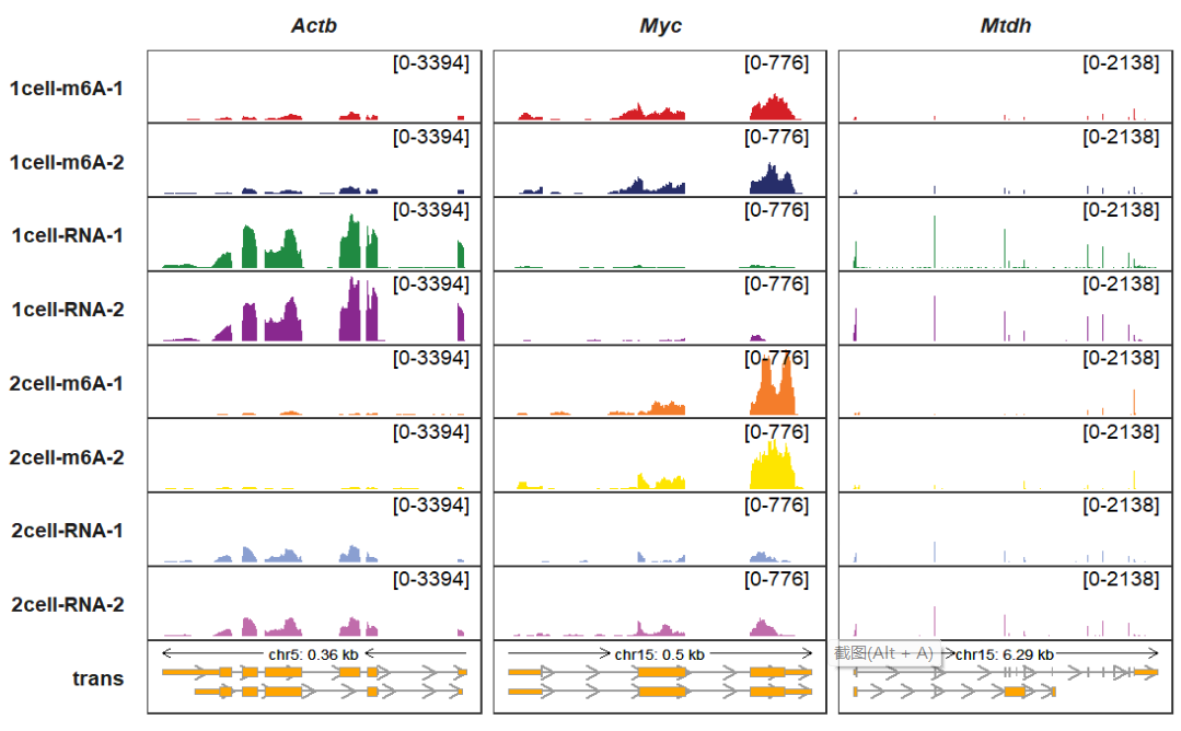
Changing arrow colors:
trackVisProMax(Input_gtf = gtf,
               Input_bw = bw,
               Input_gene = c("Actb","Myc","Mtdh"),
               trans_exon_col_params = list(fill = "black",color = "black"))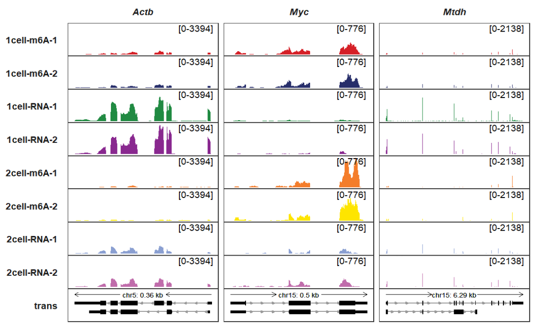
add_gene_label_layer allows you to mark gene symbols beside the transcript:
trackVisProMax(Input_gtf = gtf,
               Input_bw = bw,
               Input_gene = c("Actb","Myc","Mtdh"),
               collapse_trans = T,
               add_gene_label_layer = T,
               gene_label_shift_y = -0.5)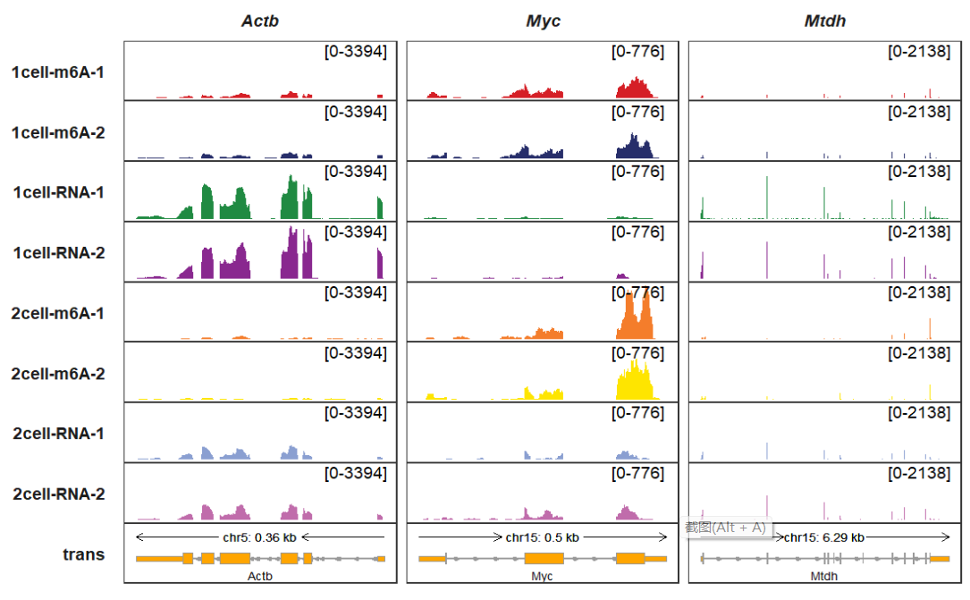
exon_width allows you to change exon width:
trackVisProMax(Input_gtf = gtf,
               Input_bw = bw,
               Input_gene = c("Actb","Myc","Mtdh"),
               exon_width = 0.9)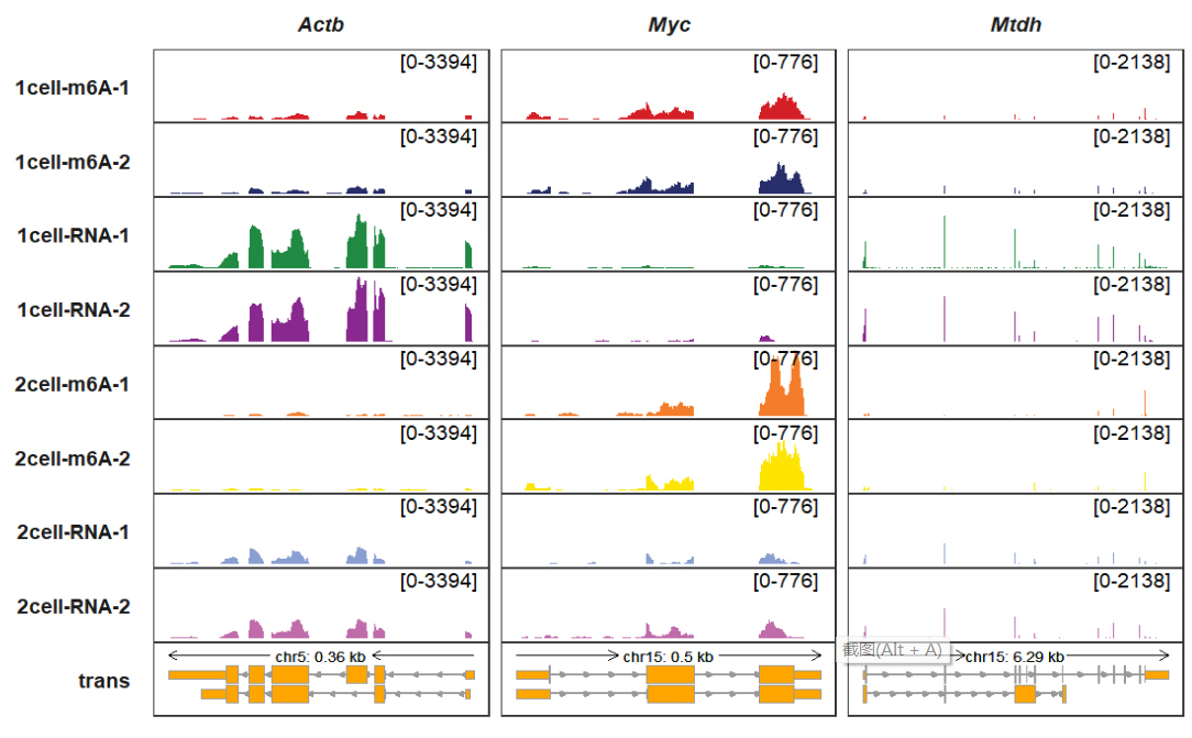
gene_dist_mark_params and gene_dist_mark_text_params control the segment (arrow direction stands for transciption direction) and chromosome label styles upper the transcript:
trackVisProMax(Input_gtf = gtf,
               Input_bw = bw,
               Input_gene = c("Actb","Myc"),
               gene_dist_mark_params = list(color = "blue",size = 1),
               gene_dist_mark_text_params = list(color = "red",size = 2))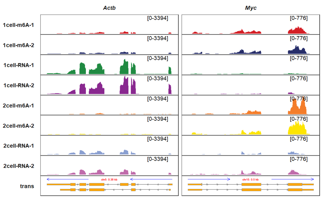
Viewing transcript structures for gene if you do not supply with any signal data (bigwig,peaks …):
Showing all transcripts:
Collapsing all transcripts:
trackVisProMax(Input_gtf = gtf,
               Input_gene = c("Dnaaf5","Zfp68","Pabpc1"),
               trans_topN = "all",
               collapse_trans = T)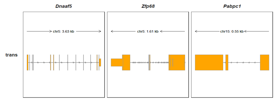
Plotting in a genomic region:
trackVisProMax(Input_gtf = gtf,
               query_region = list(query_chr = c("5","15"),
                                   query_start = c(65438603,9263295),
                                   query_end = c(65834288,9785835)))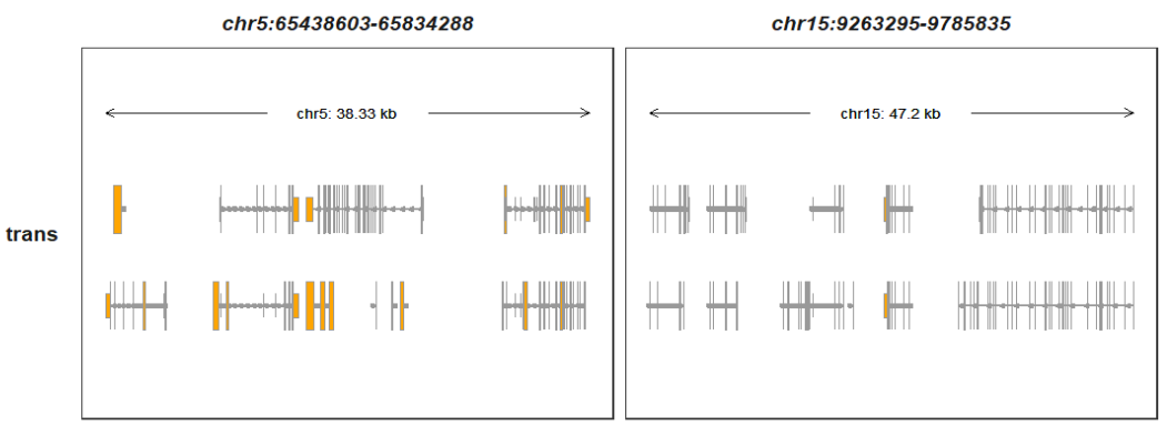
Showing all transcripts:
trackVisProMax(Input_gtf = gtf,
               query_region = list(query_chr = c("5","15"),
                                   query_start = c(65438603,9263295),
                                   query_end = c(65834288,9785835)),
               trans_topN = "all")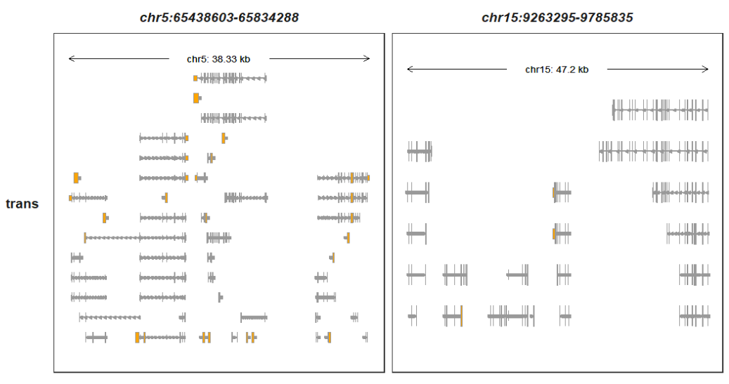
You can also map the exon color into different feature types:
# gtf
raw_gtf <- rtracklayer::import.gff("test-bw2/hg19.ncbiRefSeq.gtf.gz",format = "gtf") %>%
  data.frame()

trackVisProMax(Input_gtf = raw_gtf,
               Input_gene = c("MYC","NANOG","MALAT1"),
               trans_topN = "all",
               trans_exon_col_params = list(mapping = aes(fill = type)))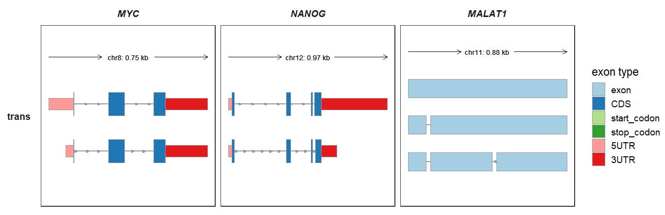
trans_fill_col accepts a character vectors or named vectors to control exon fill colors:
trackVisProMax(Input_gtf = raw_gtf,
               Input_gene = c("MYC","NANOG","MALAT1"),
               trans_topN = "all",
               trans_exon_col_params = list(mapping = aes(fill = type)),
               trans_fill_col = ggsci::pal_igv()(6))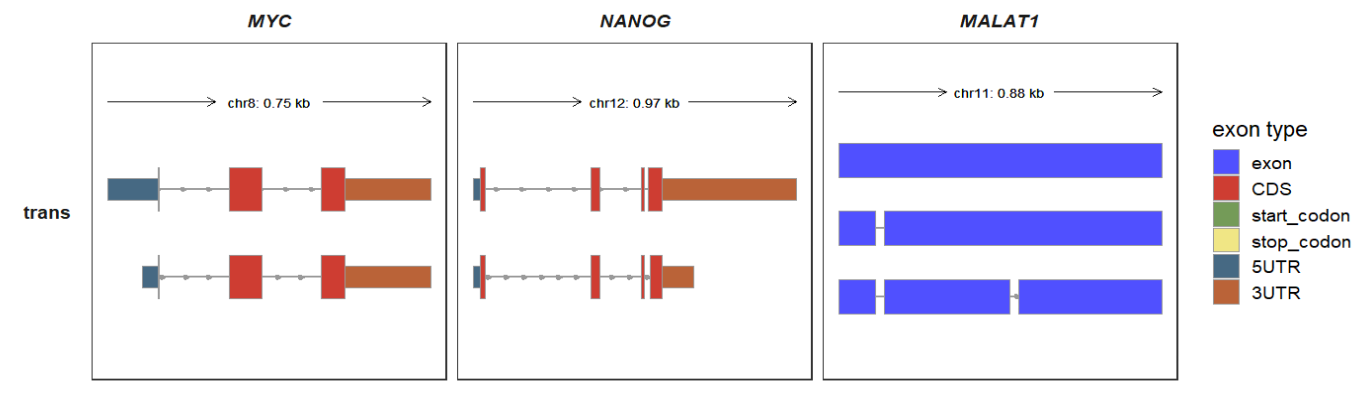
Removing the legend:
trackVisProMax(Input_gtf = raw_gtf,
               Input_gene = c("MYC","NANOG","MALAT1"),
               trans_topN = "all",
               trans_exon_col_params = list(mapping = aes(fill = type),
                                            show.legend = F),
               trans_fill_col = ggsci::pal_locuszoom()(6))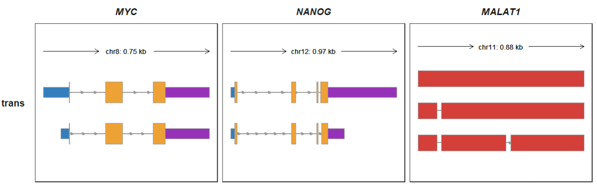
5.4 Intron line type
Intron_line_type allows you to change the intron line type(default “line”):
gtf <- rtracklayer::import.gff("Homo_sapiens.GRCh38.106.gtf.gz") %>%
  data.frame()

trackVisProMax(Input_gtf = gtf,
               Input_gene = c("ACTB","NANOG","YTHDF2"),
               Intron_line_type = "chevron")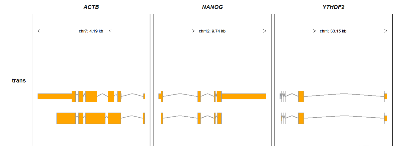
5.5 X axis limitation
Basiclly trackVisProMax is constructed based on the ggplot. But you can’t directlly use ggplot2::xlim function to adjust the X axis limitation. xlimit_range parameter is supplied to control the X axis limits which can zoom your interested region:
trackVisProMax(Input_gtf = gtf,
               Input_bw = bw,
               Input_gene = c("Actb","Myc"),
               xlimit_range = list(c(142904344,142904782),
                                   c(61987507,61988278)))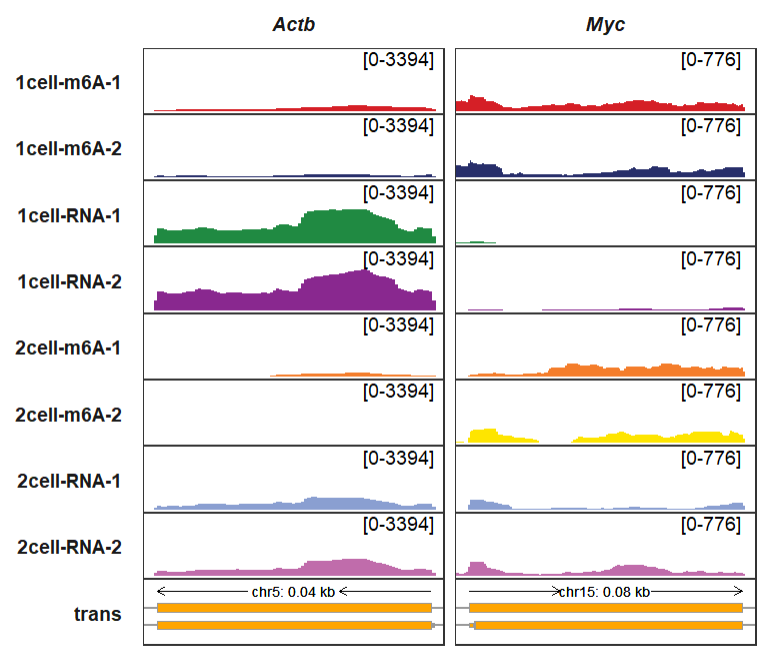
5.6 Background and highlight region settings
Maybe you need to highlight some regions where you are interested in or set background color for each track to enhance the track visualization or for other purpose. Let’s show some examples with this goal.
background_color_region accepts a named list with named vectors to control the background colors for each panel:
sample <- c("1cell-m6A-1","1cell-m6A-2","1cell-RNA-1","1cell-RNA-2",
            "2cell-m6A-1","2cell-m6A-2","2cell-RNA-1","2cell-RNA-2")

Actb_col <- rep(ggsci::pal_npg()(4),each = 2)
names(Actb_col) <- sample
Actb_col
# 1cell-m6A-1 1cell-m6A-2 1cell-RNA-1 1cell-RNA-2 2cell-m6A-1 2cell-m6A-2 2cell-RNA-1 2cell-RNA-2
# "#E64B35FF" "#E64B35FF" "#4DBBD5FF" "#4DBBD5FF" "#00A087FF" "#00A087FF" "#3C5488FF" "#3C5488FF"

Myc_col <- rep(ggsci::pal_d3()(4),each = 2)
names(Myc_col) <- sample
Myc_col
# 1cell-m6A-1 1cell-m6A-2 1cell-RNA-1 1cell-RNA-2 2cell-m6A-1 2cell-m6A-2 2cell-RNA-1 2cell-RNA-2
# "#1F77B4FF" "#1F77B4FF" "#FF7F0EFF" "#FF7F0EFF" "#2CA02CFF" "#2CA02CFF" "#D62728FF" "#D62728FF"

Mtdh_col <- rep(ggsci::pal_lancet()(4),each = 2)
names(Mtdh_col) <- sample
Mtdh_col
# 1cell-m6A-1 1cell-m6A-2 1cell-RNA-1 1cell-RNA-2 2cell-m6A-1 2cell-m6A-2 2cell-RNA-1 2cell-RNA-2
# "#00468BFF" "#00468BFF" "#ED0000FF" "#ED0000FF" "#42B540FF" "#42B540FF" "#0099B4FF" "#0099B4FF"

trackVisProMax(Input_gtf = gtf,
               Input_bw = bw,
               Input_gene = c("Actb","Myc","Mtdh"),
               background_color_region = list(Actb = Actb_col,
                                              Myc = Myc_col,
                                              Mtdh = Mtdh_col))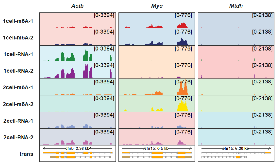
You can also set a background color for a specified panel:
trackVisProMax(Input_gtf = gtf,
               Input_bw = bw,
               Input_gene = c("Actb","Myc","Mtdh"),
               background_color_region = list(Myc = Myc_col))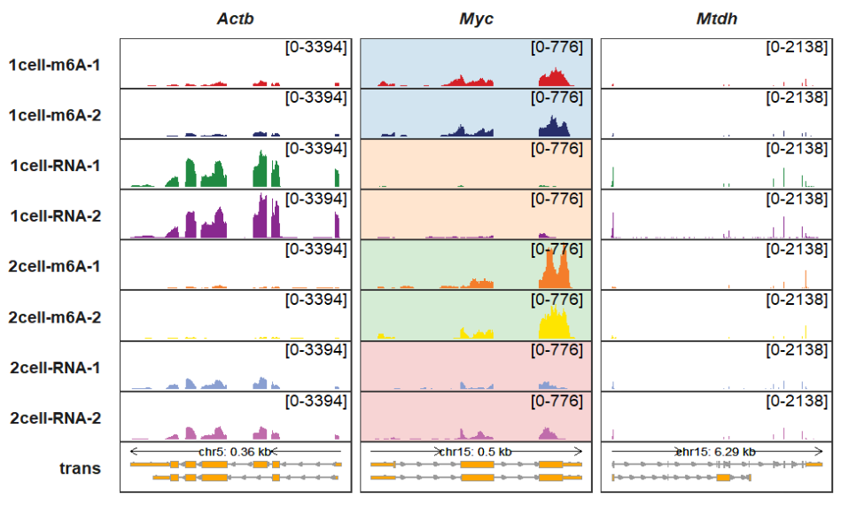
background_region_alpha controls the color transparency:
trackVisProMax(Input_gtf = gtf,
               Input_bw = bw,
               Input_gene = c("Actb","Myc","Mtdh"),
               background_color_region = list(Actb = Actb_col,
                                              Myc = Myc_col,
                                              Mtdh = Mtdh_col),
               background_region_alpha = 0.75)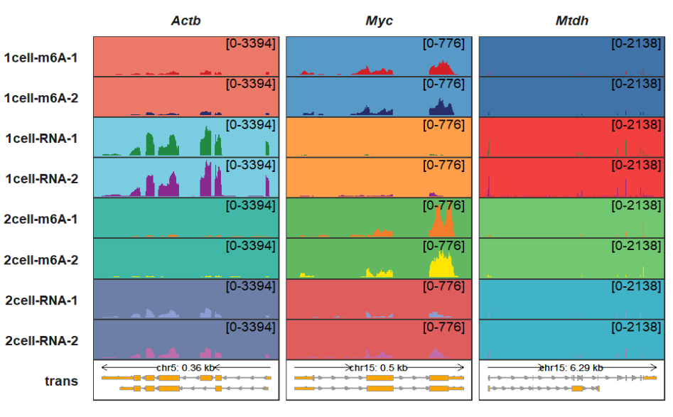
higlight_region accepts a named list genomic coordinates where you want to highlight. higlight_col also accepts a named list to control the highlighted region colors:
higlight_region <- list(Actb = list(start = c(142904000),
                                    end = c(142904500)),
                        Myc = list(start = c(61986000,61989500),
                                   end = c(61986500,61989900)))

higlight_col <- list(Actb = c("pink"),
                     Myc = c("orange","green"))

trackVisProMax(Input_gtf = gtf,
               Input_bw = bw,
               Input_gene = c("Actb","Myc","Mtdh"),
               higlight_region = higlight_region,
               higlight_col = higlight_col)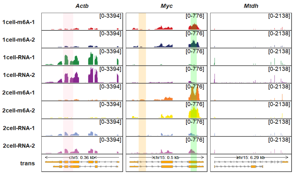
higlight_col_alpha controls the color transparency:
trackVisProMax(Input_gtf = gtf,
               Input_bw = bw,
               Input_gene = c("Actb","Myc","Mtdh"),
               higlight_region = higlight_region,
               higlight_col = higlight_col,
               higlight_col_alpha = 0.5)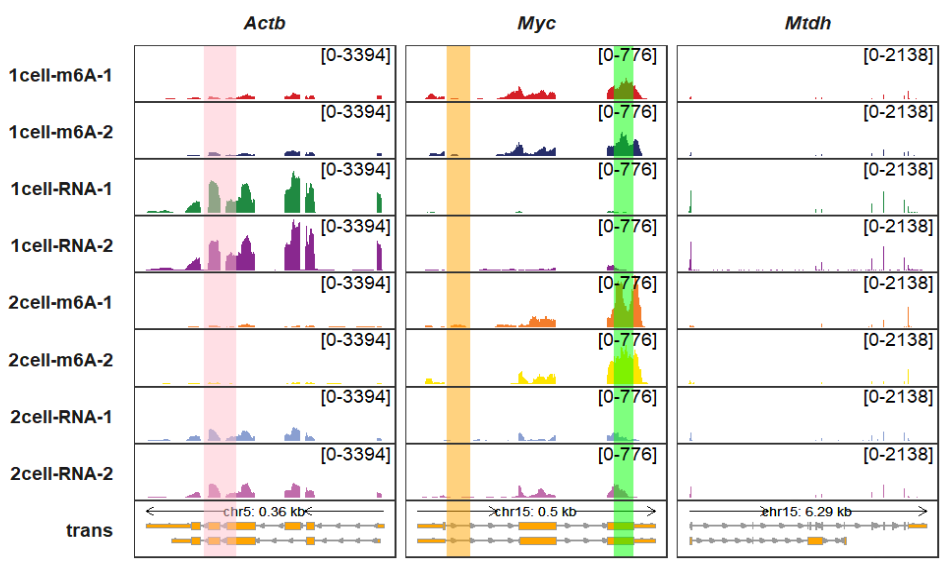
5.7 Order for genes and samples
Probably you will re-order your gene or sample orders in the graph. Generally speaking, whether the gene orders or sample orders, their orders initially have been assigned according to their input orders. You just need to adjust the input orders. Even so, I also supply gene_order and sample_order extra parameters to re-order the genes and samples:
trackVisProMax(Input_gtf = gtf,
Input_bw = bw,
Input_gene = c("Actb","Myc","Mtdh"),
gene_order = c("Mtdh","Myc","Actb"))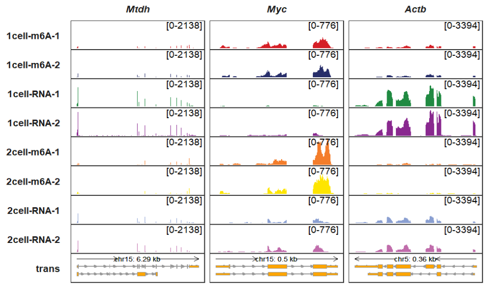 Changing sample orders:
trackVisProMax(Input_gtf = gtf,
               Input_bw = bw,
               Input_gene = c("Actb","Myc","Mtdh"),
               gene_order = c("Mtdh","Myc","Actb"),
               sample_order = rev(sample))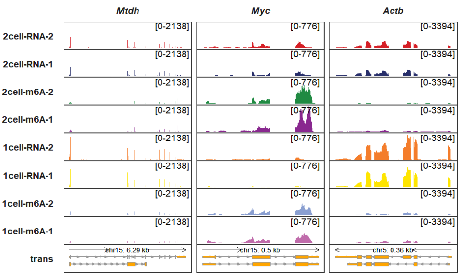
5.8 Adding group information for genes and samples
Grouping the genes and samples can clarify author’s experiment design in different conditions or treatment. So drawing group graphic elements for multiple genes or samples stands for what the author want to express. A picture is worth a thousand words.
gene_group_info, gene_group_info2,sample_group_info and sample_group_info2 accepts a named list with vectors to add group information.
You can add two group information for genes and samples at most which is enough for us. The following codes show how we add group information and modify graphic attributes.
trackVisProMax(Input_gtf = gtf,
               Input_bw = bw,
               Input_gene = c("Actb","Myc","Mtdh","Adamts3","Zfp68","Pabpc1"),
               gene_group_info = list(cluster1 = c("Actb","Myc"),
                                      cluster2 = c("Mtdh","Adamts3"),
                                      cluster3 = c("Zfp68","Pabpc1")))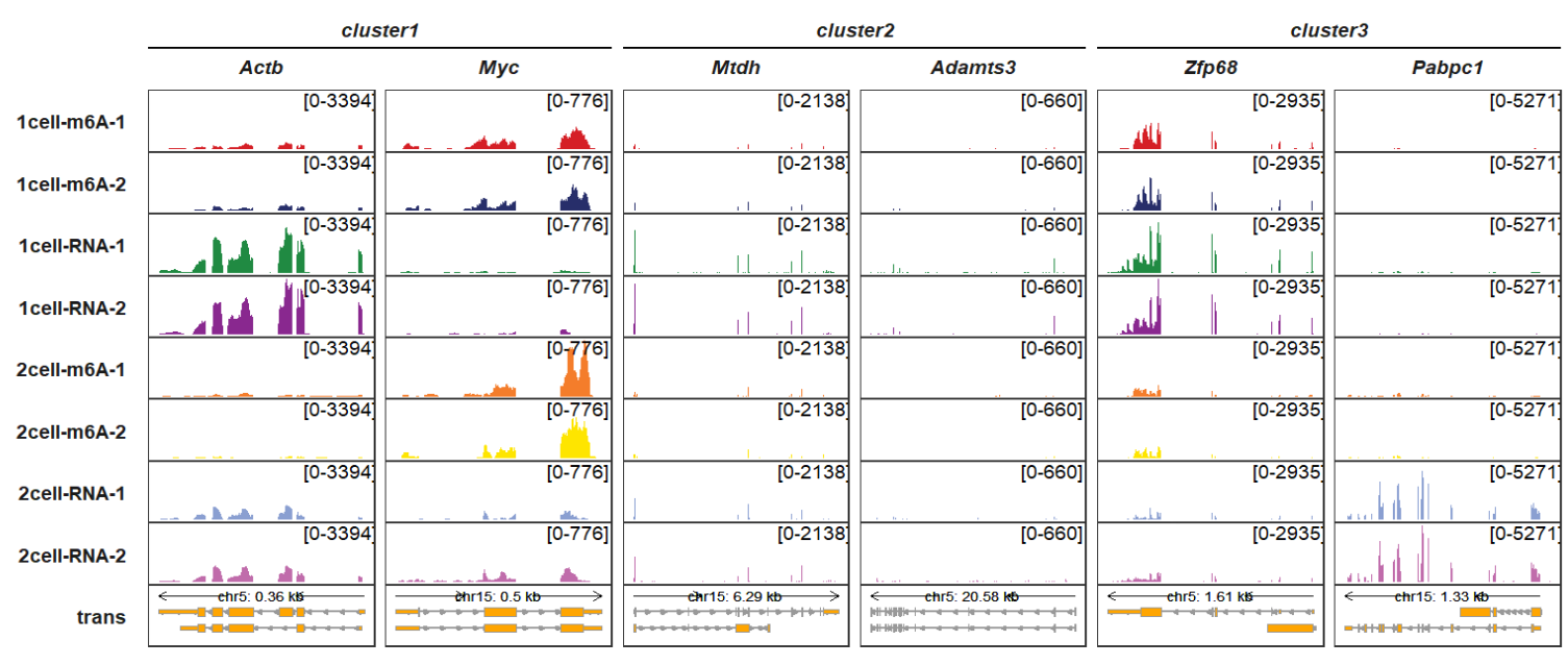
Adding sample group information:
Note: panel.spacing is used to add spacing between each panel along the Y axis which can show the line gaps between different sample group.
trackVisProMax(Input_gtf = gtf,
               Input_bw = bw,
               Input_gene = c("Actb","Myc","Mtdh","Adamts3","Zfp68","Pabpc1"),
               gene_group_info = list(cluster1 = c("Actb","Myc"),
                                      cluster2 = c("Mtdh","Adamts3"),
                                      cluster3 = c("Zfp68","Pabpc1")),
               sample_group_info = list("input" = c("1cell-RNA-1", "1cell-RNA-2",
                                                    "2cell-RNA-1", "2cell-RNA-2"),
                                        "treat" = c("1cell-m6A-1", "1cell-m6A-2",
                                                    "2cell-m6A-1", "2cell-m6A-2")),
               panel.spacing = c(0.2,0.2))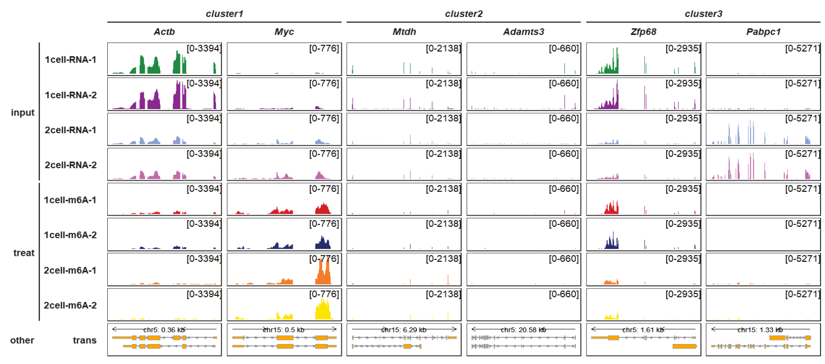
Adding one more group:
trackVisProMax(Input_gtf = gtf,
               Input_bw = bw,
               Input_gene = c("Actb","Myc","Mtdh","Adamts3","Zfp68","Pabpc1"),
               gene_group_info = list(cluster1 = c("Actb","Myc"),
                                      cluster2 = c("Mtdh","Adamts3"),
                                      cluster3 = c("Zfp68","Pabpc1")),
               gene_group_info2 = list(geneGroup1 = c("Actb","Myc","Mtdh"),
                                       geneGroup2 = c("Adamts3","Zfp68","Pabpc1")),
               sample_group_info = list("input" = c("1cell-RNA-1", "1cell-RNA-2",
                                                    "2cell-RNA-1", "2cell-RNA-2"),
                                        "treat" = c("1cell-m6A-1", "1cell-m6A-2",
                                                    "2cell-m6A-1", "2cell-m6A-2")),
               sample_group_info2 = list("cellState1" = c("1cell-RNA-1", "1cell-RNA-2",
                                                          "1cell-m6A-1", "1cell-m6A-2"),
                                         "cellState2" = c("2cell-RNA-1", "2cell-RNA-2",
                                                          "2cell-m6A-1", "2cell-m6A-2")),
               panel.spacing = c(0.2,0.2))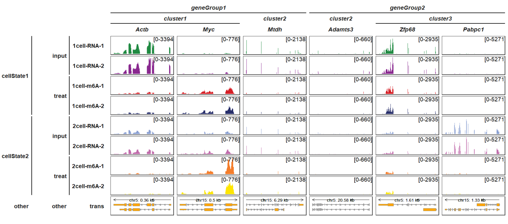
gene_group_info_order, gene_group_info2_order,sample_group_info_order and sample_group_info2_order separatelly control each group orders:
trackVisProMax(Input_gtf = gtf,
               Input_bw = bw,
               Input_gene = c("Actb","Myc","Mtdh","Adamts3","Zfp68","Pabpc1"),
               gene_group_info = list(cluster1 = c("Actb","Myc"),
                                      cluster2 = c("Mtdh","Adamts3"),
                                      cluster3 = c("Zfp68","Pabpc1")),
               gene_group_info_order = c("cluster3","cluster2","cluster1"),
               gene_group_info2 = list(geneGroup1 = c("Actb","Myc","Mtdh"),
                                       geneGroup2 = c("Adamts3","Zfp68","Pabpc1")),
               gene_group_info2_order = c("geneGroup2","geneGroup1"),
               sample_group_info = list("input" = c("1cell-RNA-1", "1cell-RNA-2",
                                                    "2cell-RNA-1", "2cell-RNA-2"),
                                        "treat" = c("1cell-m6A-1", "1cell-m6A-2",
                                                    "2cell-m6A-1", "2cell-m6A-2")),
               sample_group_info_order = c("treat","input"),
               sample_group_info2 = list("cellState1" = c("1cell-RNA-1", "1cell-RNA-2",
                                                          "1cell-m6A-1", "1cell-m6A-2"),
                                         "cellState2" = c("2cell-RNA-1", "2cell-RNA-2",
                                                          "2cell-m6A-1", "2cell-m6A-2")),
               sample_group_info2_order = c("cellState2","cellState1"),
               panel.spacing = c(0.2,0.2))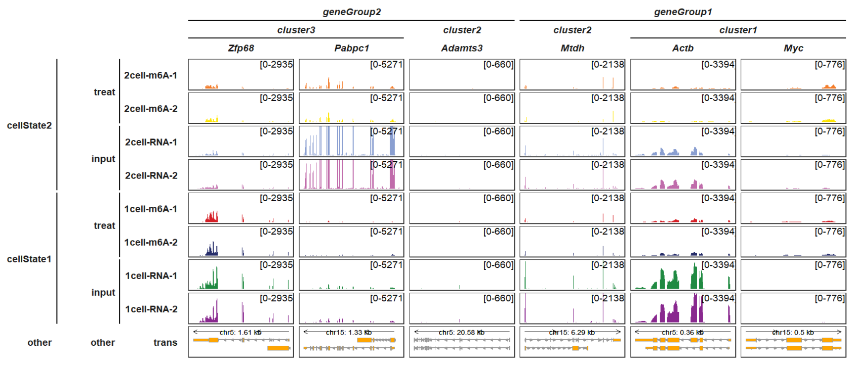
5.9 Strip settings
This chapter shows us how to modify each strip graphic element instead of using lines to separate group.
column_strip_setting_list and row_strip_setting_list accept a named list to modify the strip element_rect element by columns or rows:
trackVisProMax(Input_gtf = gtf,
               Input_bw = bw,
               Input_gene = c("Actb","Myc","Mtdh"),
               column_strip_setting_list = list(color = rep("red",3),
                                                fill = rep("grey80",3)),
               row_strip_setting_list = list(color = rep("black",8),
                                             fill = rep(c("orange","purple"),each = c(2,2),
                                                        times = 2)))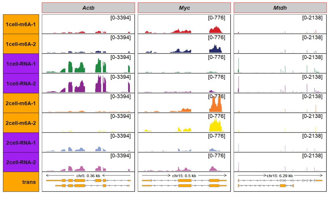
column_strip_text_setting_list and row_strip_text_setting_list accept a named list to modify the strip element_text element by columns or rows:
trackVisProMax(Input_gtf = gtf,
               Input_bw = bw,
               Input_gene = c("Actb","Myc","Mtdh"),
               column_strip_setting_list = list(color = rep("red",3),
                                                fill = rep("grey80",3)),
               column_strip_text_setting_list = list(color = "darkred",size = 8,
                                                     fontface = "bold"),
               row_strip_setting_list = list(color = rep("black",8),
                                             fill = rep(c("orange","purple"),each = c(2,2),
                                                        times = 2)),
               row_strip_text_setting_list = list(fontface = "italic.bold",color = "white"))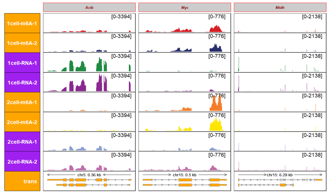
by_layer_x and by_layer_y can be setted to TRUE and you can modify the graphic element by row or column:
trackVisProMax(Input_gtf = gtf,
               Input_bw = bw,
               Input_gene = c("Actb","Myc","Mtdh","Adamts3","Zfp68","Pabpc1"),
               gene_group_info = list(cluster1 = c("Actb","Myc"),
                                      cluster2 = c("Mtdh","Adamts3"),
                                      cluster3 = c("Zfp68","Pabpc1")),
               gene_group_info2 = list(geneGroup1 = c("Actb","Myc","Mtdh"),
                                       geneGroup2 = c("Adamts3","Zfp68","Pabpc1")),
               by_layer_x = T,
               column_strip_setting_list = list(fill = c("grey80","blue","green")),
               sample_group_info = list("input" = c("1cell-RNA-1", "1cell-RNA-2",
                                                    "2cell-RNA-1", "2cell-RNA-2"),
                                        "treat" = c("1cell-m6A-1", "1cell-m6A-2",
                                                    "2cell-m6A-1", "2cell-m6A-2")),
               sample_group_info2 = list("cellState1" = c("1cell-RNA-1", "1cell-RNA-2",
                                                          "1cell-m6A-1", "1cell-m6A-2"),
                                         "cellState2" = c("2cell-RNA-1", "2cell-RNA-2",
                                                          "2cell-m6A-1", "2cell-m6A-2")),
               by_layer_y = T,
               row_strip_setting_list = list(fill = c("purple","yellow","pink")),
               panel.spacing = c(0.2,0.2))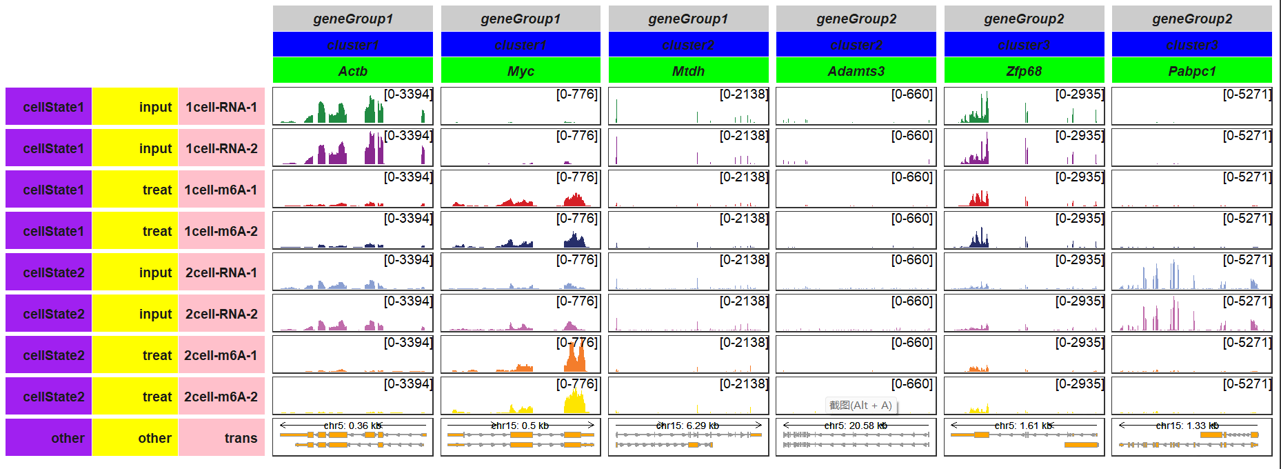
- More details you can check ggh4x::strip_themed function.
5.10 Draw chromosome annotation
Here you can add corresponding genome ideogram data to show chromosome structure for gene. First you should load ideogram data. The are some prepared genome like mm10, hg39, hg19 can be loaded to use directly. For other genome versions, you can use BioSeqUtils::catchIdeoData function to download it.
The catchIdeoData returns a list object:
data("mm10_obj")

str(mm10_obj)
# List of 3
# $ plot_df     :'data.frame':  403 obs. of  6 variables:
#   ..$ chr        : chr [1:403] "chr1" "chr1" "chr1" "chr1" ...
# ..$ chromStart : num [1:403] 0 8840440 12278390 20136559 22101102 ...
# ..$ chromEnd   : num [1:403] 8840440 12278390 20136559 22101102 30941543 ...
# ..$ name       : chr [1:403] "qA1" "qA2" "qA3" "qA4" ...
# ..$ gieStain   : chr [1:403] "gpos100" "gneg" "gpos33" "gneg" ...
# ..$ gieStainCol: chr [1:403] "black" "white" "gray67" "white" ...
# $ border_df   : tibble [21 × 3] (S3: tbl_df/tbl/data.frame)
# ..$ chr : chr [1:21] "chr1" "chr10" "chr11" "chr12" ...
# ..$ xmin: num [1:21] 0 0 0 0 0 0 0 0 0 0 ...
# ..$ xmax: num [1:21] 1.95e+08 1.31e+08 1.22e+08 1.20e+08 1.20e+08 ...
# $ acen_plot_df: NULL
draw_chromosome should be setted to TRUE if you want to add chromosome facet annotation. draw_chromosome_params accepts a named list to control how the chromosome structure is drawn. More details please refer to BioSeqUtils::drawChromosome function. Now we add chromosome facet track for corresponding genes:
trackVisProMax(Input_gtf = gtf,
               Input_bw = bw,
               Input_gene = c("Actb","Myc","Mtdh","Adamts3"),
               draw_chromosome = T,
               draw_chromosome_params = list(ideogram_obj = mm10_obj))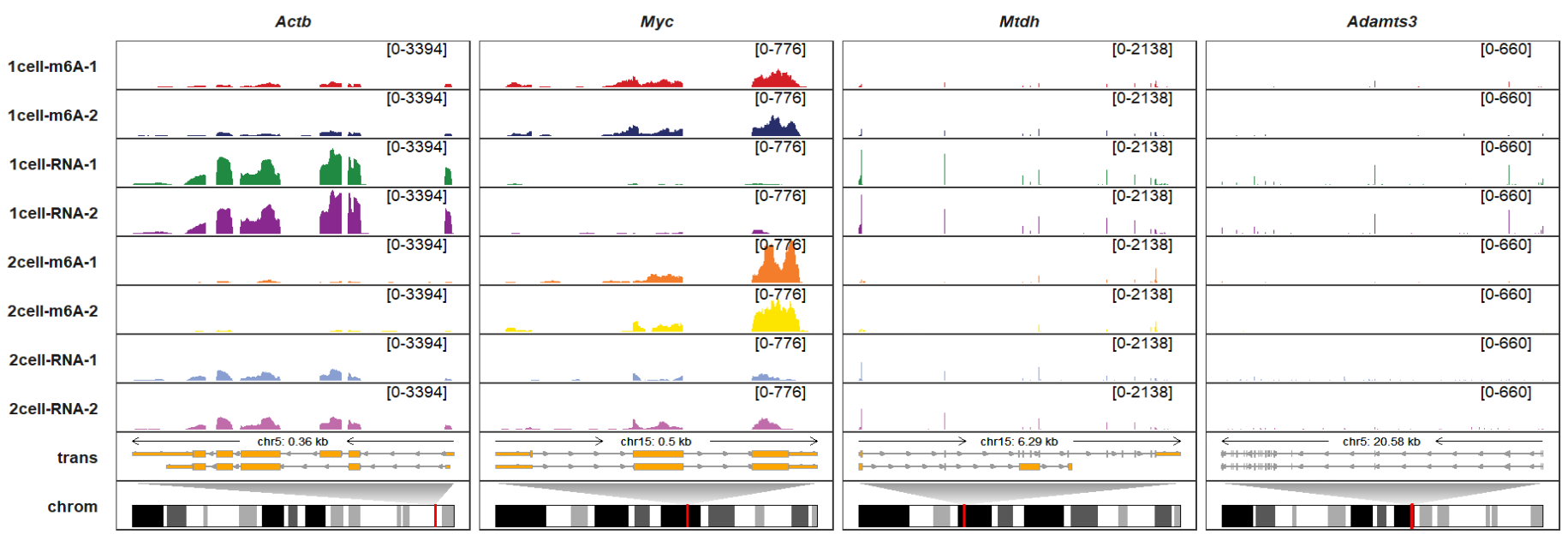
remove_chrom_panel_border can be used to remove chromosome track panel borders:
trackVisProMax(Input_gtf = gtf,
               Input_bw = bw,
               Input_gene = c("Actb","Myc","Mtdh","Adamts3"),
               draw_chromosome = T,
               draw_chromosome_params = list(ideogram_obj = mm10_obj),
               remove_chrom_panel_border = T)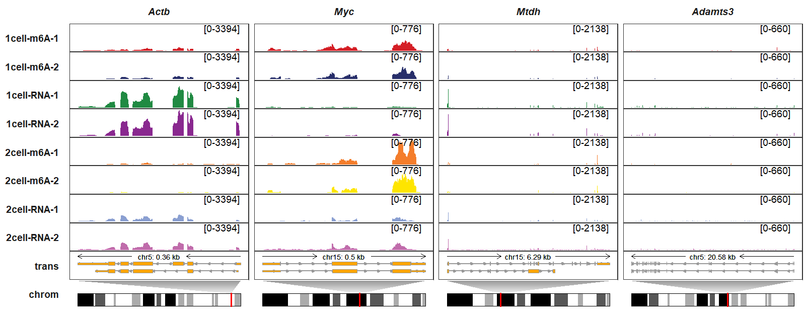
You can also use remove_all_panel_border to remove all track panel borders with more concise presentation:
trackVisProMax(Input_gtf = gtf,
               Input_bw = bw,
               Input_gene = c("Actb","Myc","Mtdh","Adamts3"),
               draw_chromosome = T,
               draw_chromosome_params = list(ideogram_obj = mm10_obj),
               remove_all_panel_border = T)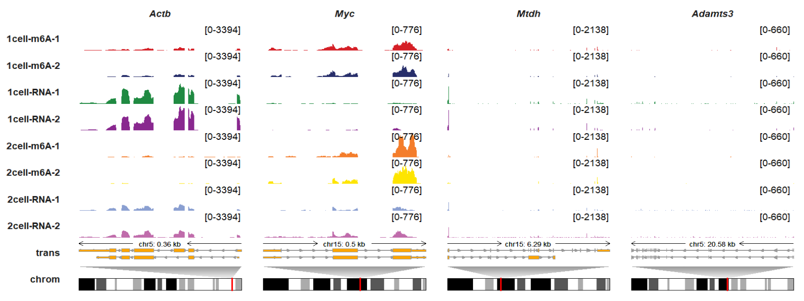
panel_size_setting allows you to set width and height for each panel. Here we reduce the chromosome panel height:
trackVisProMax(Input_gtf = gtf,
               Input_bw = bw,
               Input_gene = c("Actb","Myc","Mtdh","Adamts3"),
               draw_chromosome = T,
               draw_chromosome_params = list(ideogram_obj = mm10_obj),
               remove_chrom_panel_border = T,
               panel_size_setting = list(rows = rep(c(4,4,4,4,4,4,4,4,4,2),4),
                                         cols = rep(12,4)))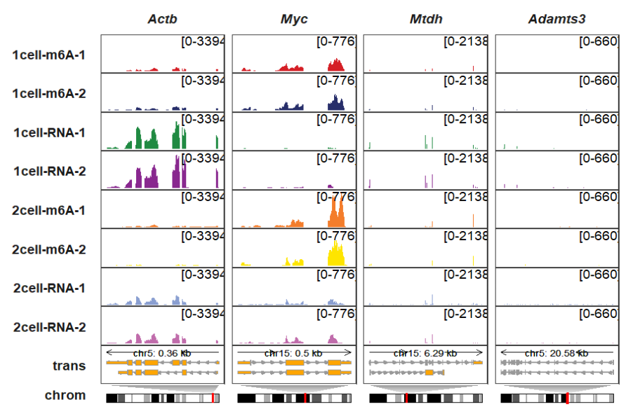
Let’s add some group informations:
trackVisProMax(Input_gtf = gtf,
               Input_bw = bw,
               Input_gene = c("Actb","Myc","Mtdh","Adamts3"),
               draw_chromosome = T,
               draw_chromosome_params = list(ideogram_obj = mm10_obj),
               remove_chrom_panel_border = T,
               panel_size_setting = list(rows = rep(c(4,4,4,4,4,4,4,4,4,2),4),
                                         cols = rep(12,4)),
               gene_group_info = list(cluster1 = c("Actb","Myc"),
                                      cluster2 = c("Mtdh","Adamts3"),
                                      cluster3 = c("Zfp68","Pabpc1")),
               sample_group_info = list("input" = c("1cell-RNA-1", "1cell-RNA-2",
                                                    "2cell-RNA-1", "2cell-RNA-2"),
                                        "treat" = c("1cell-m6A-1", "1cell-m6A-2",
                                                    "2cell-m6A-1", "2cell-m6A-2")),
               panel.spacing = c(0.2,0.2))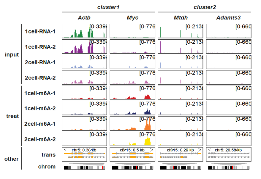
5.11 Plot with specified genomic region
Maybe sometimes we need to show the track information with given a specified genomic region instead of genes. You can give a named list for query_region to draw different genomic region tracks. Multiple genomic positions also can be accepted.
Examples show here:
trackVisProMax(Input_gtf = gtf,
               Input_bw = bw,
               query_region = list(query_chr = c("5","15"),
                                   query_start = c(65438603,9263295),
                                   query_end = c(65834288,9785835)))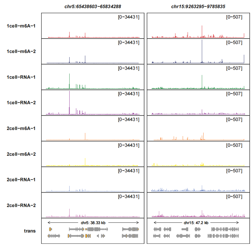
Modifing the transcript arrow styles and show all trancripts:
trackVisProMax(Input_gtf = gtf,
               Input_bw = bw,
               query_region = list(query_chr = c("5","15"),
                                   query_start = c(65438603,9263295),
                                   query_end = c(65834288,9785835)),
               trans_topN = "all",
               fixed_column_range = F,
               trans_exon_arrow_params = list(arrow = arrow(length = unit(0.3,"mm")),
                                              linewidth = 0.2))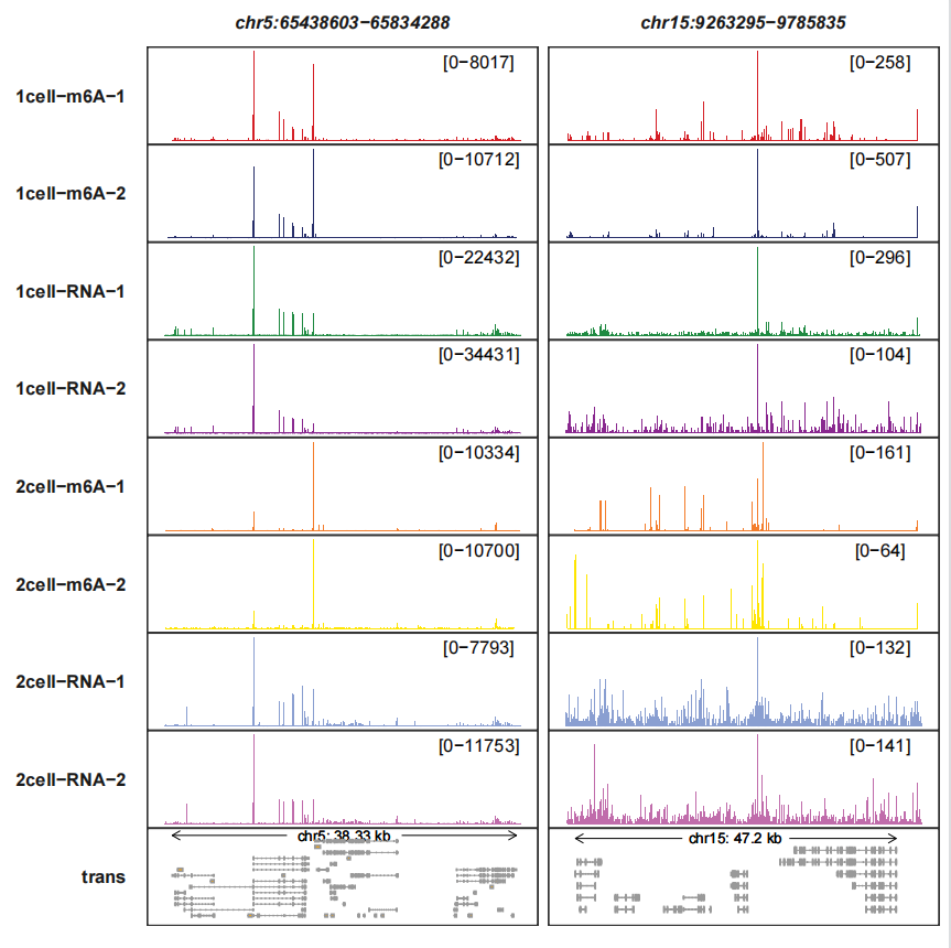
The details for trans track:
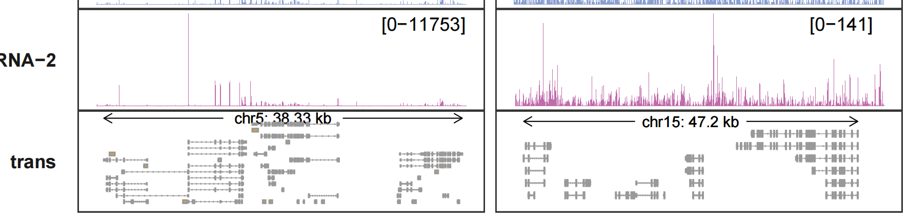
Adding gene labels:
trackVisProMax(Input_gtf = gtf,
               Input_bw = bw,
               query_region = list(query_chr = c("5","15"),
                                   query_start = c(65438603,9263295),
                                   query_end = c(65834288,9785835)),
               trans_topN = "all",
               fixed_column_range = F,
               trans_exon_arrow_params = list(arrow = arrow(length = unit(0.3,"mm")),
                                              linewidth = 0.2),
               add_gene_label_layer = T,
               gene_label_params = list(size = 1,segment.size = 0.1))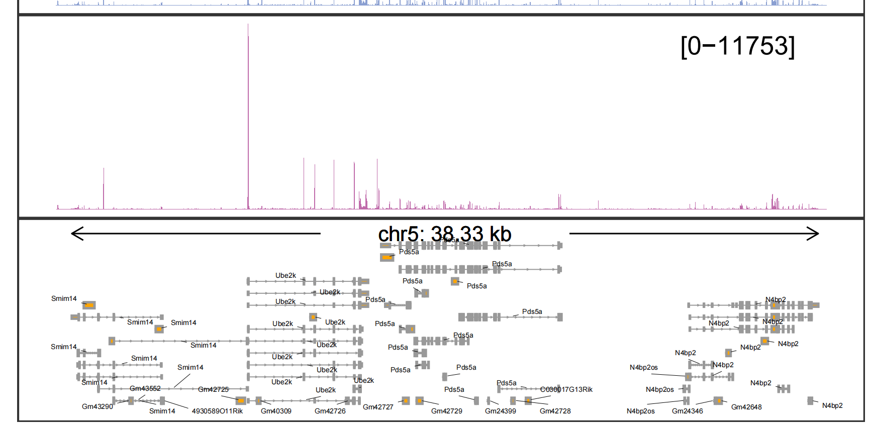
Collapsing transcripts:
trackVisProMax(Input_gtf = gtf,
               Input_bw = bw,
               query_region = list(query_chr = c("5","15"),
                                   query_start = c(65438603,9263295),
                                   query_end = c(65834288,9785835)),
               collapse_trans = T,
               fixed_column_range = F,
               trans_exon_arrow_params = list(arrow = arrow(length = unit(0.3,"mm")),
                                              linewidth = 0.2),
               add_gene_label_layer = T,
               gene_label_params = list(size = 1,segment.size = 0.1),
               gene_label_shift_y = -0.5)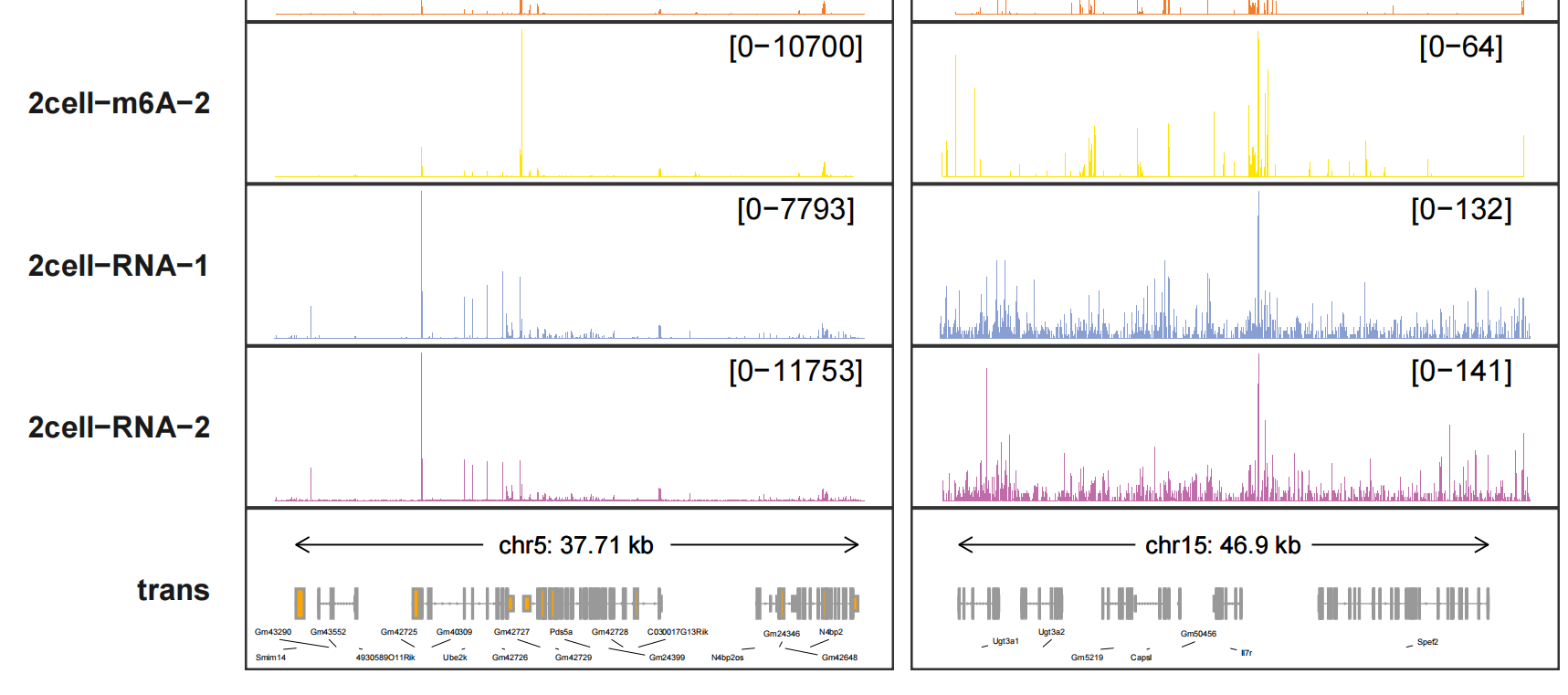
Adding chromosome structure:
trackVisProMax(Input_gtf = gtf,
               Input_bw = bw,
               query_region = list(query_chr = c("5","15"),
                                   query_start = c(65438603,9263295),
                                   query_end = c(65834288,9785835)),
               trans_topN = "all",
               fixed_column_range = F,
               trans_exon_arrow_params = list(arrow = arrow(length = unit(0.3,"mm")),
                                              linewidth = 0.2),
               add_gene_label_layer = T,
               gene_label_params = list(size = 1,segment.size = 0.1),
               draw_chromosome = T,
               draw_chromosome_params = list(ideogram_obj = mm10_obj))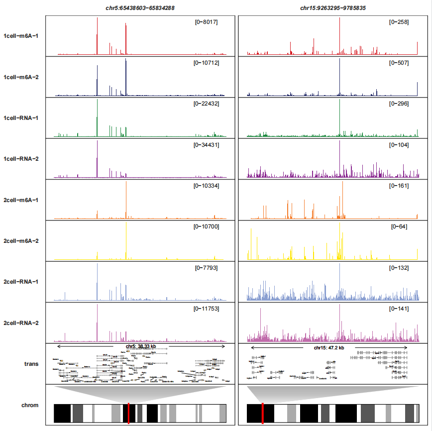
5.12 Adding peaks track
I don’t draw the peaks file to assign each new panel. I have put them all into one panel which is enough. This is similar with the trans panel. Input_bed accepts peaks data which output from loadBed function. We first load the peaks data:
bedfile <- list.files(path = "./",pattern = ".bed")
# [1] "peaks.bed"  "peaks2.bed"

bed_df <- loadBed(bedfile)

# check
head(bed_df,3)
#   seqnames     start       end sampleName y
# 1        5 142905501 142905600      peaks 1
# 2        5 142903201 142903800      peaks 1
# 3       15  61985342  61985900      peaks 1
Plotting the peaks track:
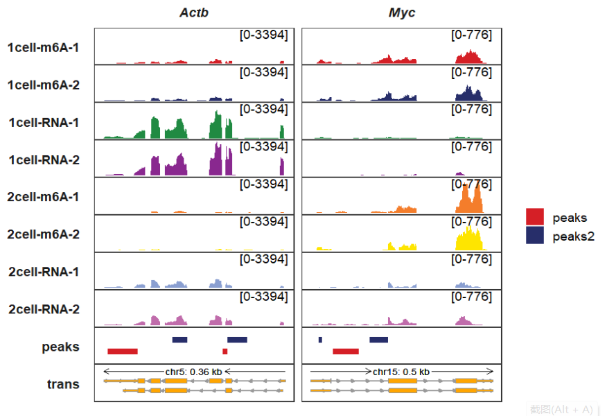
peak_width controls the peaks rectangle height:
trackVisProMax(Input_gtf = gtf,
               Input_bw = bw,
               Input_bed = bed_df,
               Input_gene = c("Actb","Myc"),
               peak_width = 0.9)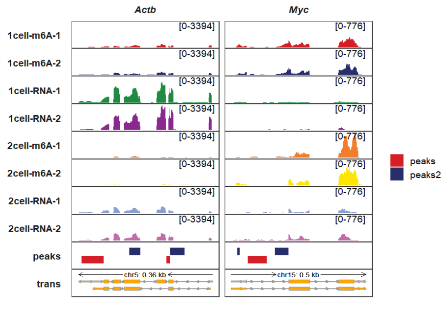
peak_fill_col controls the peaks rectangle colors:
trackVisProMax(Input_gtf = gtf,
               Input_bw = bw,
               Input_bed = bed_df,
               Input_gene = c("Actb","Myc"),
               peak_width = 0.9,
               peak_fill_col = c(peaks = "orange",peaks2 = "purple"))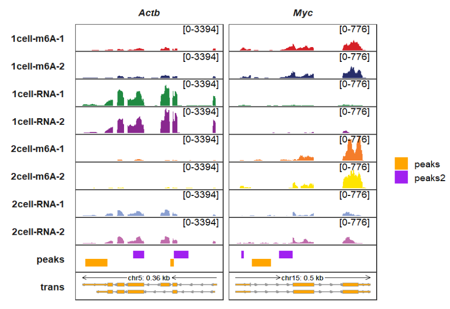
Adding chromosomes:
trackVisProMax(Input_gtf = gtf,
               Input_bw = bw,
               Input_bed = bed_df,
               Input_gene = c("Actb","Myc"),
               peak_width = 0.9,
               peak_fill_col = c(peaks = "orange",peaks2 = "purple"),
               draw_chromosome = T,
               draw_chromosome_params = list(ideogram_obj = mm10_obj))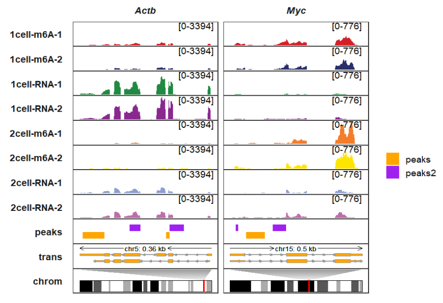
5.13 Extending bases upstream and downstream
Drawing specific genes and observe the signals sometimes are not enough. Finding the transcription factor binding signals for gene upstream is what we want. It is not simple to supply exact genomic coordinates to draw. upstream_extend and downstream_extend allow you to extend bases upstream or downstream for your genes, here we show some examples:
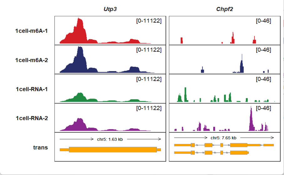
Extending upstream:
trackVisProMax(Input_gtf = gtf,
               Input_bw = bw,
               Input_gene = c("Utp3","Chpf2"),
               upstream_extend = 2000)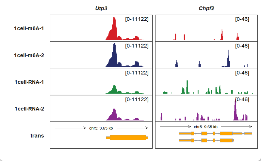
Extending upstream and downstream:
trackVisProMax(Input_gtf = gtf,
               Input_bw = bw,
               Input_gene = c("Utp3","Chpf2"),
               upstream_extend = 2000,
               downstream_extend = 2000)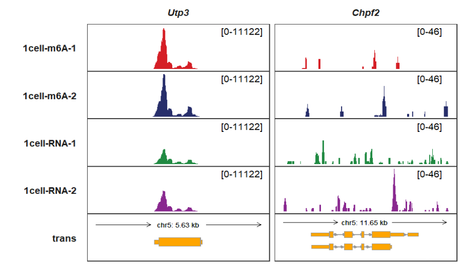
You can extend for multiple genes with different values:
trackVisProMax(Input_gtf = gtf,
               Input_bw = bw,
               Input_gene = c("Utp3","Chpf2"),
               upstream_extend = c(2000,1000),
               downstream_extend = c(1000,2000)
               )