Chapter 9 Other funs

9.1 Transcript coordinate transformation

Mostly we draw transcript structures on genomic coordinates which contain intron sequence. Sometimes you just want to compare multiple transcripts for a gene with removing introns. transCoordTransform allows you to transform the genomic coordinate into absolute coordinate from gtf file.

Here are the examples:

library(patchwork)

# gtf
raw_gtf <- rtracklayer::import.gff("test-bw2/hg19.ncbiRefSeq.gtf.gz",format = "gtf") %>% 
  data.frame() 

p1 <-
trackVisProMax(Input_gtf = raw_gtf,
               Input_gene = c("MYC","NANOG"))

p1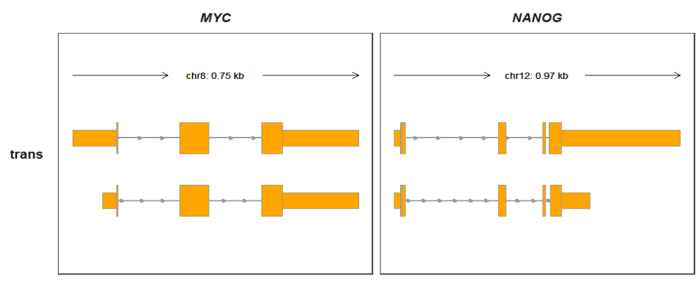

Transforming coordinate:

tgene <- raw_gtf %>% filter(gene_name %in% c("MYC","NANOG"))

trans_gtf <- transCoordTransform(gtf_file = tgene)

# check
head(trans_gtf[1:3,1:8])
#   seqnames start  end width strand                source       type score
# 1    chr12     1 2049  6660      + ncbiRefSeq.2021-05-17 transcript    NA
# 2    chr12     1  364   364      + ncbiRefSeq.2021-05-17       exon    NA
# 3    chr12   365  627   263      + ncbiRefSeq.2021-05-17       exon    NA

p2 <-
trackVisProMax(Input_gtf = trans_gtf,
               Input_gene = c("MYC","NANOG"))

p2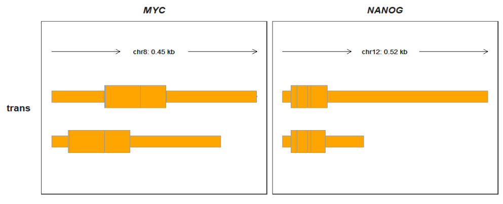

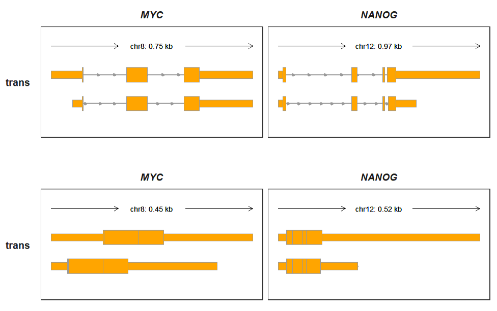
p1/p2

p3 <- 
trackVisProMax(Input_gtf = trans_gtf,
               Input_gene = c("MYC","NANOG"),
               trans_exon_col_params = list(mapping = aes(fill = type)))

p1/p2/p3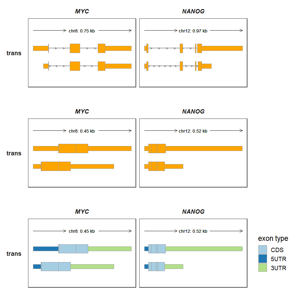

9.2 Track overlap

For some experiments, you got IP(immunoprecipitation) and Input group, maybe you need to put them together to compare difference of signals. One way we can assign a new fileName column and set fill colors with your experiment groups. Examples showed here:

---

First we assign new columns for bigwig data:

library(BioSeqUtils)
library(ggplot2)

# load bigwig files
file <- list.files(path = "test-bw/",pattern = '.bw',full.names = T)
file
# [1] "test-bw/1cell-m6A-1.bw" "test-bw/1cell-m6A-2.bw" "test-bw/1cell-RNA-1.bw"
# [4] "test-bw/1cell-RNA-2.bw" "test-bw/2cell-m6A-1.bw" "test-bw/2cell-m6A-2.bw"
# [7] "test-bw/2cell-RNA-1.bw" "test-bw/2cell-RNA-2.bw"

# select some chromosomes for test
bw <- loadBigWig(file,chrom = c("5","15"))

# check
head(bw,3)
#   seqnames   start     end   score    fileName
# 1       15       1 3054635 0.00000 1cell-m6A-1
# 2       15 3054636 3054640 1.34079 1cell-m6A-1
# 3       15 3054641 3054715 2.68159 1cell-m6A-1

bw_new <- bw
bw_new$new_name <- paste(sapply(strsplit(bw_new$fileName,split = "-"),"[",1),
                         sapply(strsplit(bw_new$fileName,split = "-"),"[",3),sep = "-")

bw_new$exptype <- sapply(strsplit(bw_new$fileName,split = "-"),"[",2)

bw_new$fileName <- bw_new$new_name

# order
bw$exptype <- factor(bw$exptype,levels = c("m6A","RNA"))

# check
head(bw_new)
#   seqnames   start     end   score fileName new_name exptype
# 1       15       1 3054635 0.00000  1cell-1  1cell-1     m6A
# 2       15 3054636 3054640 1.34079  1cell-1  1cell-1     m6A
# 3       15 3054641 3054715 2.68159  1cell-1  1cell-1     m6A
# 4       15 3054716 3054720 1.34079  1cell-1  1cell-1     m6A
# 5       15 3054721 3060760 0.00000  1cell-1  1cell-1     m6A
# 6       15 3060761 3060765 1.34079  1cell-1  1cell-1     m6A


# gtf
gtf <- rtracklayer::import.gff("Mus_musculus.GRCm38.102.gtf",format = "gtf") %>% 
  data.frame()

Plot for all samples:

trackVisProMax(Input_gtf = gtf,
               Input_bw = bw,
               Input_gene = c("Utp3","Chpf2","Dmp1"))

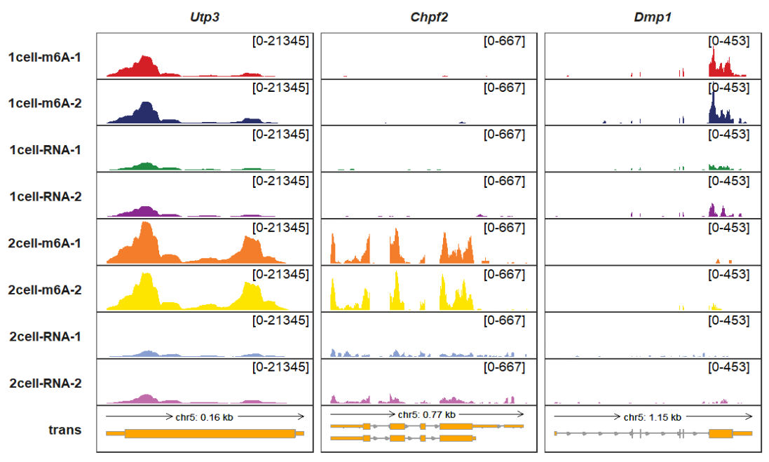
Plot for overlap tracks, we can see the difference of ip(m6A) and input(RNA) better:

# plot
trackVisProMax(Input_gtf = gtf,
               Input_bw = bw_new,
               Input_gene = c("Utp3","Chpf2","Dmp1"),
               signal_layer_bw_params = list(mapping = aes(fill = exptype,color = exptype),
                                             show.legend = T))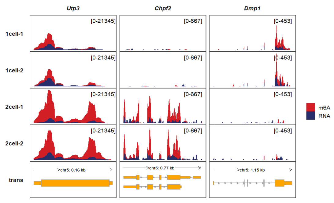

9.3 Extend coordinate for gene

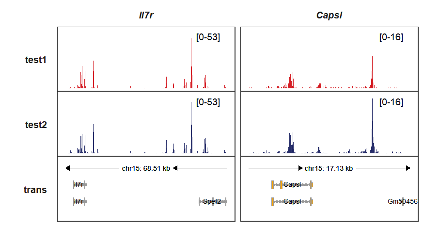
You may want to extend to a specific coordinate when you plot track for a gene, such as focus on near the TSS(transcript start site). xlimit_range can be defined with exact genomic coordinate for each gene.

Let’s show whole the gene structures:

# load bigwig files
file <- list.files(path = "../bw/",pattern = '.bw',full.names = T)
file

# select some chromosomes for test
bw <- loadBigWig(bw_file = file[1:2],chrom = c("chr15"),format = "bw",file_name = c("test1","test2"))

# check
head(bw,3)

# gtf
my_gtf <- rtracklayer::import.gff("../Mus_musculus.GRCm38.102.gtf.gz",format = "gtf") %>%
  data.frame()
my_gtf$seqnames <- paste("chr",my_gtf$seqnames,sep = "")

# plot
# Il7r
trackVisProMax(Input_gtf = my_gtf,
               Input_bw = bw,
               Input_gene = c("Il7r"))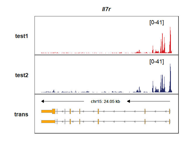

Given a specific genomic coordinate:

# 9515784-9550038
trackVisProMax(Input_gtf = my_gtf,
               Input_bw = bw,
               Input_gene = c("Il7r"),
               xlimit_range = c(9515784,9555038))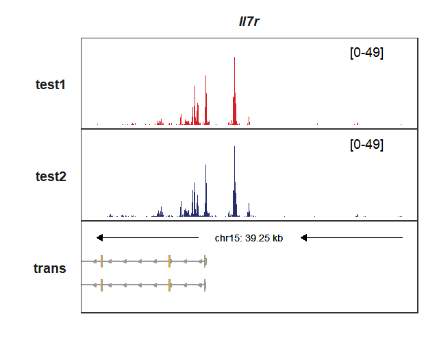

The gene structures will be shown if the genomic coordinate is out of the target gene:

# 9268339-9542382
trackVisProMax(Input_gtf = my_gtf,
               Input_bw = bw,
               Input_gene = c("Il7r"),
               xlimit_range = c(9268339,9542382))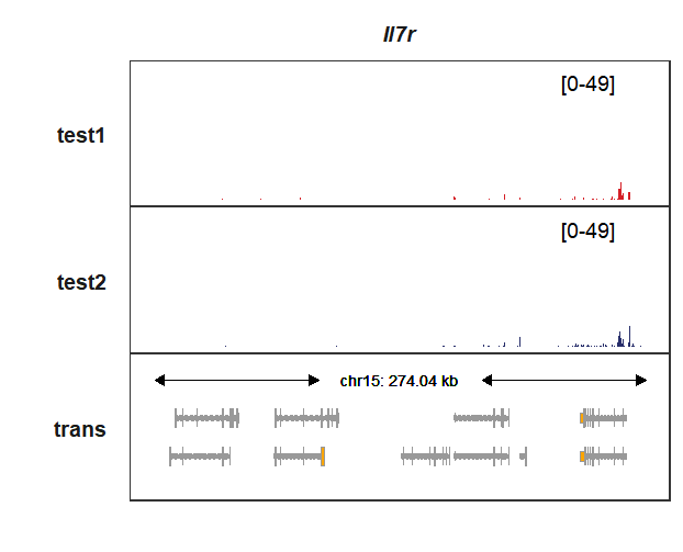

Multiple target genes with xlimit_range list:

trackVisProMax(Input_gtf = my_gtf,
               Input_bw = bw,
               Input_gene = c("Il7r","Capsl"),
               add_gene_label_layer = T,
               xlimit_range = list(c(9521626,9590136),c(9459212,9476339))
)