Chapter 6 Loops visualization
For Hi-C, HiChIP and ChIA-PET sequencing technologies, them aim to catch the three dimension interaction of chromosomes. Finding interaction sites and visualize them which are on demand. Usually we use arch links to represent the interaction information.
6.1 Input data prepration
Test data can be fetched on GSE200165.
We can use loadloops function to load the interaction sites data:
loop_file <- list.files("test-bw2/",pattern = ".bedpe$",full.names = T)
loop_file
# [1] "test-bw2/C1-CTCF.bedpe"    "test-bw2/C1-H3K27ac.bedpe" "test-bw2/M1-CTCF.bedpe"
# [4] "test-bw2/M1-H3K27ac.bedpe"

file_name = c("C1-CTCF","C1-H3K27ac","M1-CTCF","M1-H3K27ac")

# test code
loop_data <- loadloops(loop_file = loop_file,file_name = file_name,
                       sep = " ")

# check
head(loop_data,3)

#   seqnames     start       end    score fileName
# 1    chr10 100002774 100022436 0.021354  C1-CTCF
# 2    chr10 100002774 100069170 0.068404  C1-CTCF
# 3    chr10 100002774 100185646 0.184670  C1-CTCF
Test data can be fetched on GSE200160.
Here we also load bigwig data:
# bigwig
file <- list.files(path = "test-bw2/",pattern = '.bw',full.names = T)
# [1] "test-bw2/ChIP-CTCF-MYC1.bw"    "test-bw2/ChIP-H3K27ac-MYC1.bw" "test-bw2/ChIP-Input-MYC1.bw"
# [4] "test-bw2/ChIP-MYC-MYC1.bw"

bw <- loadBigWig(bw_file = file,chrom = "8")
bw$seqnames <- paste("chr",bw$seqnames,sep = "")

# gtf
gtf <- rtracklayer::import.gff("test-bw2/hg19.ncbiRefSeq.gtf.gz",format = "gtf") %>%
  data.frame()
6.2 Basic loops visualization
The legend score means the distance across two interaction sites. The higher score, the longer distance:
trackVisProMax(Input_bw = bw,
               Input_gtf = gtf,
               query_region = list(query_chr = "chr8",
                                   query_start = 100010290,
                                   query_end = 101157229),
               Input_loop = loop_data,
               fixed_column_range = F)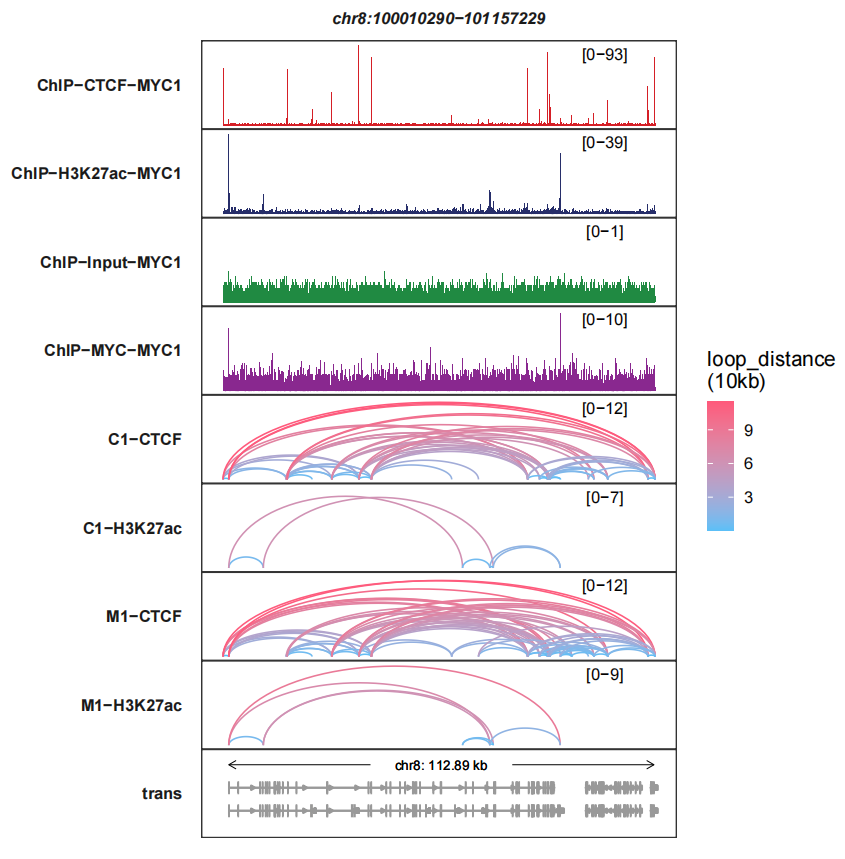
loops_col controls the color or links:
trackVisProMax(Input_bw = bw,
               Input_gtf = gtf,
               query_region = list(query_chr = "chr8",
                                   query_start = 100010290,
                                   query_end = 101157229),
               Input_loop = loop_data,
               fixed_column_range = F,
               loops_col = c("white","blue"))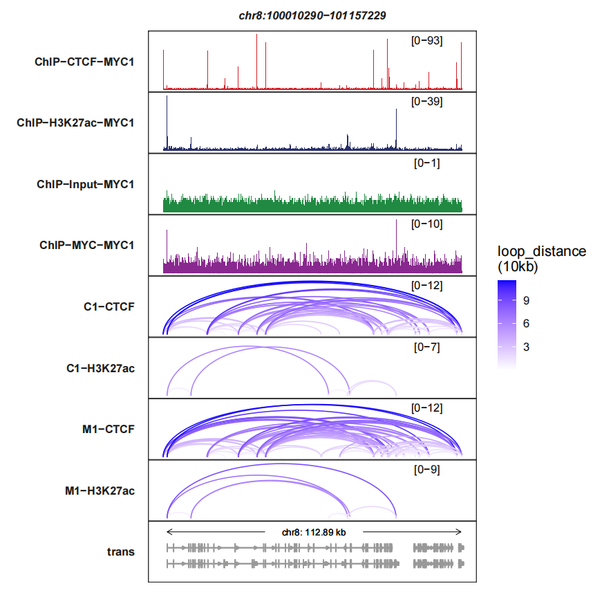
signal_layer_loop_params accepts a named list to control the links layer, For more details, please check ggbio::geom_arch. Here we turn off the legend:
trackVisProMax(Input_bw = bw,
               Input_gtf = gtf,
               query_region = list(query_chr = "chr8",
                                   query_start = 100010290,
                                   query_end = 101157229),
               Input_loop = loop_data,
               fixed_column_range = F,
               loops_col = c("white","blue"),
               signal_layer_loop_params = list(show.legend = F))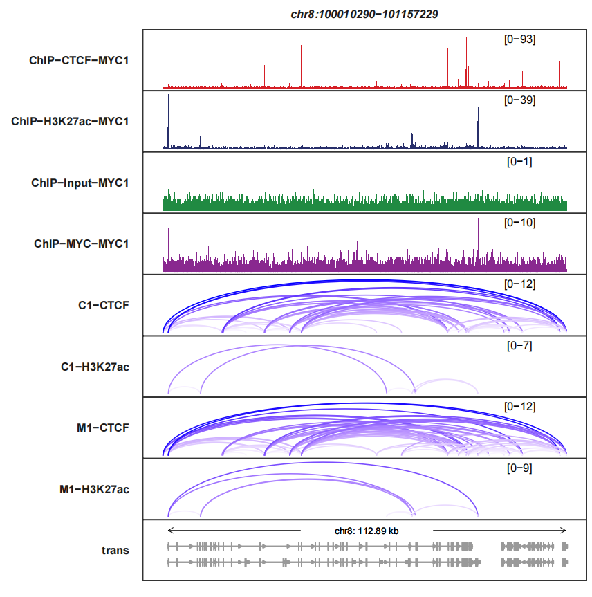
max.height can make the links panel height to be same:
trackVisProMax(Input_bw = bw,
               Input_gtf = gtf,
               query_region = list(query_chr = "chr8",
                                   query_start = 100010290,
                                   query_end = 101157229),
               Input_loop = loop_data,
               fixed_column_range = F,
               signal_layer_loop_params = list(max.height = 12))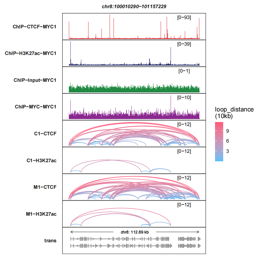
linewidth changes the links linewidth:
trackVisProMax(Input_bw = bw,
               Input_gtf = gtf,
               query_region = list(query_chr = "chr8",
                                   query_start = 100010290,
                                   query_end = 101157229),
               Input_loop = loop_data,
               fixed_column_range = F,
               signal_layer_loop_params = list(linewidth = 1))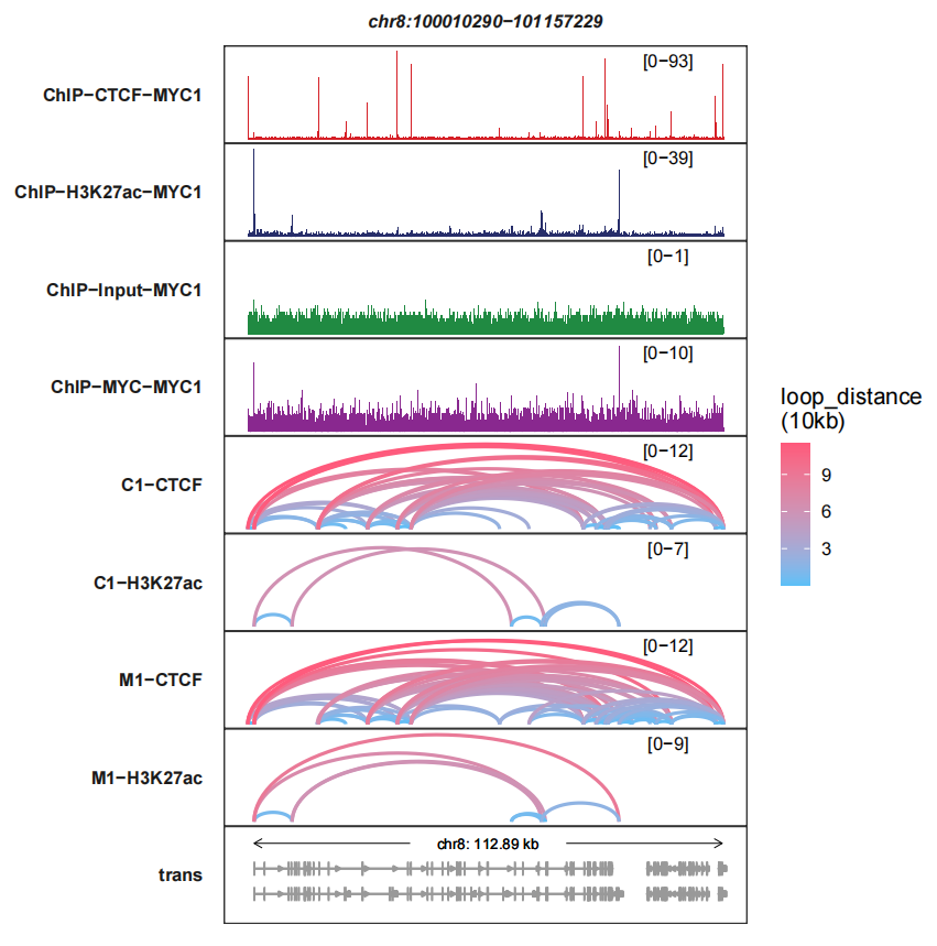
We can arrange the sample order:
trackVisProMax(Input_bw = bw,
               Input_gtf = gtf,
               query_region = list(query_chr = "chr8",
                                   query_start = 100010290,
                                   query_end = 101157229),
               Input_loop = loop_data,
               fixed_column_range = F,
               sample_order = c("M1-CTCF","ChIP-CTCF-MYC1",
                                "C1-CTCF","ChIP-MYC-MYC1",
                                "M1-H3K27ac","ChIP-H3K27ac-MYC1",
                                "C1-H3K27ac","ChIP-Input-MYC1"))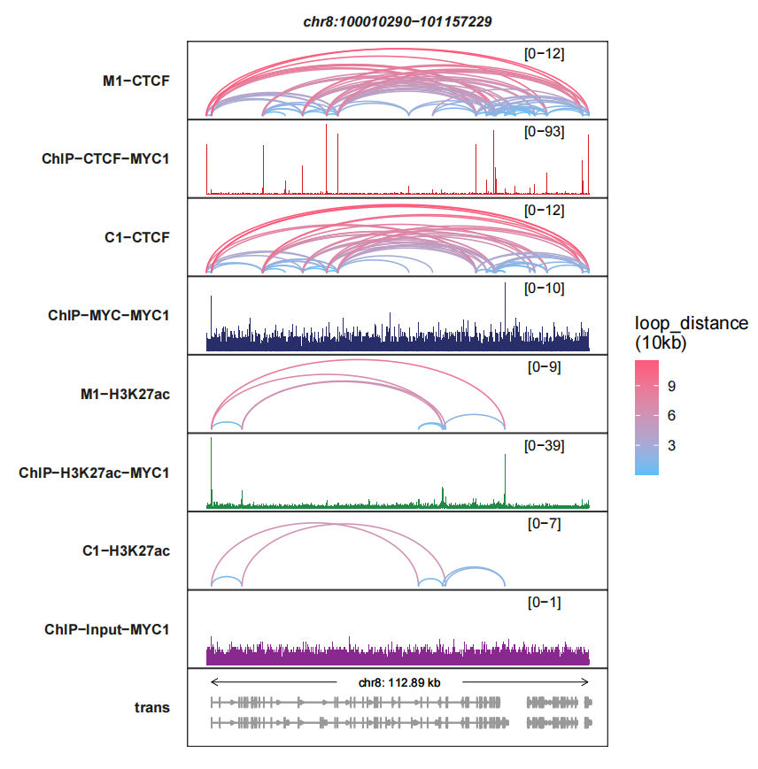
6.3 Reverse Y axis
reverse_y_vars allows you to reverse the Y axis for any signal track, you only need to give a track character name:
trackVisProMax(Input_bw = bw,
               Input_gtf = gtf,
               query_region = list(query_chr = "chr8",
                                   query_start = 100010290,
                                   query_end = 101157229),
               Input_loop = loop_data,
               fixed_column_range = F,
               sample_order = c("ChIP-CTCF-MYC1","M1-CTCF",
                                "ChIP-MYC-MYC1","C1-CTCF",
                                "ChIP-H3K27ac-MYC1","M1-H3K27ac",
                                "ChIP-Input-MYC1","C1-H3K27ac"),
               reverse_y_vars = c("M1-CTCF","C1-CTCF",
                                  "M1-H3K27ac","C1-H3K27ac"))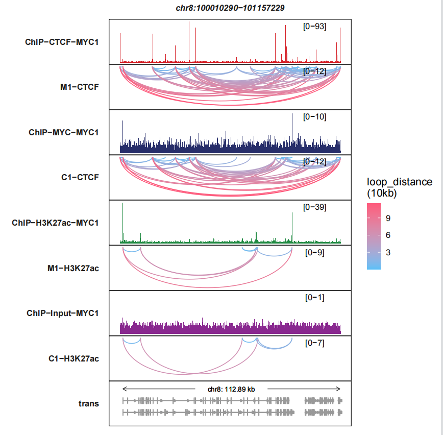
Or you can reverse the bigwig track Y axis:
trackVisProMax(Input_bw = bw,
               Input_gtf = gtf,
               query_region = list(query_chr = "chr8",
                                   query_start = 100010290,
                                   query_end = 101157229),
               Input_loop = loop_data,
               fixed_column_range = F,
               sample_order = c("M1-CTCF","ChIP-CTCF-MYC1",
                                "C1-CTCF","ChIP-MYC-MYC1",
                                "M1-H3K27ac","ChIP-H3K27ac-MYC1",
                                "C1-H3K27ac","ChIP-Input-MYC1"),
               reverse_y_vars = c("ChIP-CTCF-MYC1","ChIP-MYC-MYC1",
                                  "ChIP-H3K27ac-MYC1","ChIP-Input-MYC1"))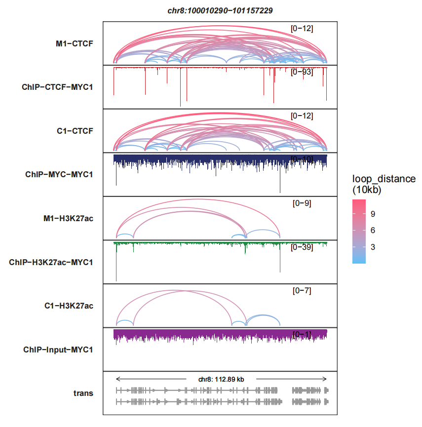
Let’s draw multiple genomic regions:
trackVisProMax(Input_bw = bw,
               Input_gtf = gtf,
               query_region = list(query_chr = c("chr8","chr8"),
                                   query_start = c(100010290,65831189),
                                   query_end = c(101157229,67351272)),
               Input_loop = loop_data,
               fixed_column_range = F,
               sample_order = c("ChIP-CTCF-MYC1","M1-CTCF",
                                "ChIP-MYC-MYC1","C1-CTCF",
                                "ChIP-H3K27ac-MYC1","M1-H3K27ac",
                                "ChIP-Input-MYC1","C1-H3K27ac"),
               reverse_y_vars = c("M1-CTCF","C1-CTCF",
                                  "M1-H3K27ac","C1-H3K27ac"))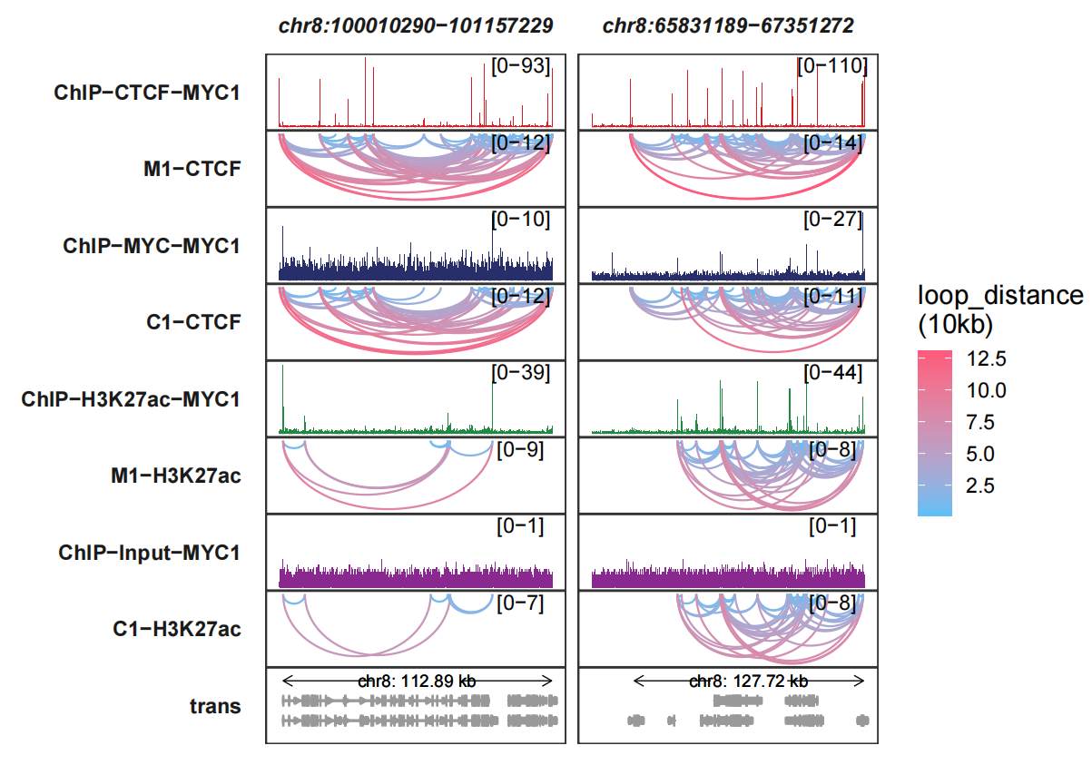
6.4 Combing with chromosome track
Adding chromosome tracks:
data("hg19_obj")
trackVisProMax(Input_bw = bw,
               Input_gtf = gtf,
               query_region = list(query_chr = c("chr8","chr8"),
                                   query_start = c(100010290,65831189),
                                   query_end = c(101157229,67351272)),
               Input_loop = loop_data,
               fixed_column_range = F,
               sample_order = c("ChIP-CTCF-MYC1","M1-CTCF",
                                "ChIP-MYC-MYC1","C1-CTCF",
                                "ChIP-H3K27ac-MYC1","M1-H3K27ac",
                                "ChIP-Input-MYC1","C1-H3K27ac"),
               reverse_y_vars = c("M1-CTCF","C1-CTCF",
                                  "M1-H3K27ac","C1-H3K27ac"),
               draw_chromosome = T,
               draw_chromosome_params = list(ideogram_obj = hg19_obj))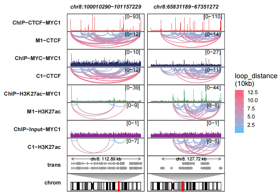
Adding group information:
trackVisProMax(Input_bw = bw,
               Input_gtf = gtf,
               query_region = list(query_chr = c("chr8","chr8"),
                                   query_start = c(100010290,65831189),
                                   query_end = c(101157229,67351272)),
               Input_loop = loop_data,
               fixed_column_range = F,
               sample_order = c("ChIP-CTCF-MYC1","M1-CTCF",
                                "ChIP-MYC-MYC1","C1-CTCF",
                                "ChIP-H3K27ac-MYC1","M1-H3K27ac",
                                "ChIP-Input-MYC1","C1-H3K27ac"),
               reverse_y_vars = c("M1-CTCF","C1-CTCF",
                                  "M1-H3K27ac","C1-H3K27ac"),
               draw_chromosome = T,
               draw_chromosome_params = list(ideogram_obj = hg19_obj),
               sample_group_info = list(state1 = c("ChIP-CTCF-MYC1","M1-CTCF"),
                                        state2 = c("ChIP-MYC-MYC1","C1-CTCF"),
                                        histoneMarker = c("ChIP-H3K27ac-MYC1","M1-H3K27ac"),
                                        inputControl = c("ChIP-Input-MYC1","C1-H3K27ac")),
               panel.spacing = c(0.2,0.2))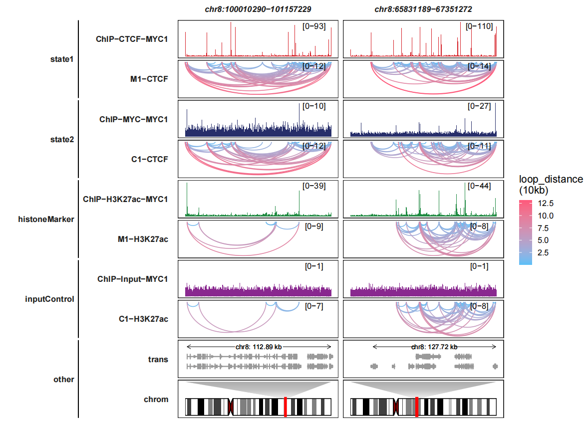
6.5 Higlight regions
Adding highlight regions:
higlight_region <- list("chr8:100010290-101157229" = list(start = c(100310290),
                                                          end = c(100457229)),
                        "chr8:65831189-67351272" = list(start = c(65931189,66231189),
                                                        end = c(66051272,66351272)))

higlight_col <- list(Actb = c("purple"),
                     Myc = c("yellow","green"))

trackVisProMax(Input_bw = bw,
               Input_gtf = gtf,
               query_region = list(query_chr = c("chr8","chr8"),
                                   query_start = c(100010290,65831189),
                                   query_end = c(101157229,67351272)),
               Input_loop = loop_data,
               fixed_column_range = F,
               sample_order = c("ChIP-CTCF-MYC1","M1-CTCF",
                                "ChIP-MYC-MYC1","C1-CTCF",
                                "ChIP-H3K27ac-MYC1","M1-H3K27ac",
                                "ChIP-Input-MYC1","C1-H3K27ac"),
               reverse_y_vars = c("M1-CTCF","C1-CTCF",
                                  "M1-H3K27ac","C1-H3K27ac"),
               draw_chromosome = T,
               draw_chromosome_params = list(ideogram_obj = hg19_obj),
               sample_group_info = list(state1 = c("ChIP-CTCF-MYC1","M1-CTCF"),
                                        state2 = c("ChIP-MYC-MYC1","C1-CTCF"),
                                        histoneMarker = c("ChIP-H3K27ac-MYC1","M1-H3K27ac"),
                                        inputControl = c("ChIP-Input-MYC1","C1-H3K27ac")),
               panel.spacing = c(0.2,0.2),
               higlight_region = higlight_region,
               higlight_col = higlight_col)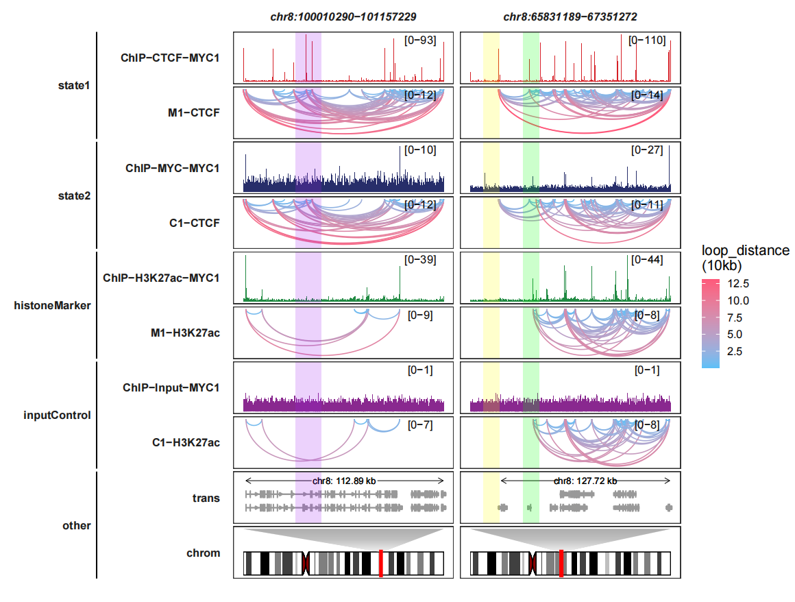
6.6 Drawing only loop tracks
We can only plot loops graph without bigwig track:
trackVisProMax(Input_gtf = gtf,
               query_region = list(query_chr = c("chr8","chr8"),
                                   query_start = c(100010290,65831189),
                                   query_end = c(101157229,67351272)),
               Input_loop = loop_data,
               fixed_column_range = F,
               draw_chromosome = T,
               draw_chromosome_params = list(ideogram_obj = hg19_obj),
               sample_group_info = list(state1 = c("C1-CTCF","M1-CTCF"),
                                        state2 = c("M1-H3K27ac","C1-H3K27ac")),
               panel.spacing = c(0.2,0.2))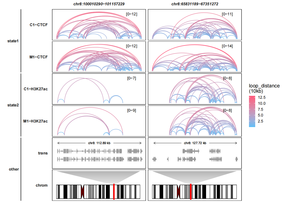
6.7 Curve geoms choosing
The curves are generated based on ggbio::geom_arch function. The curves are a little strange which means the arcs are much oblate. Here we can choose another geom layer jjPlot::geom_arch2 for better visualization. Setting Loop_curve_geom = “geom_arch2”:
trackVisProMax(Input_gtf = gtf,
               query_region = list(query_chr = c("chr8","chr8"),
                                   query_start = c(100010290,65831189),
                                   query_end = c(101157229,67351272)),
               Input_loop = loop_data,
               fixed_column_range = F,
               draw_chromosome = T,Loop_curve_geom = "geom_arch2",
               draw_chromosome_params = list(ideogram_obj = hg19_obj),
               sample_group_info = list(state1 = c("C1-CTCF","M1-CTCF"),
                                        state2 = c("M1-H3K27ac","C1-H3K27ac")),
               panel.spacing = c(0.2,0.2))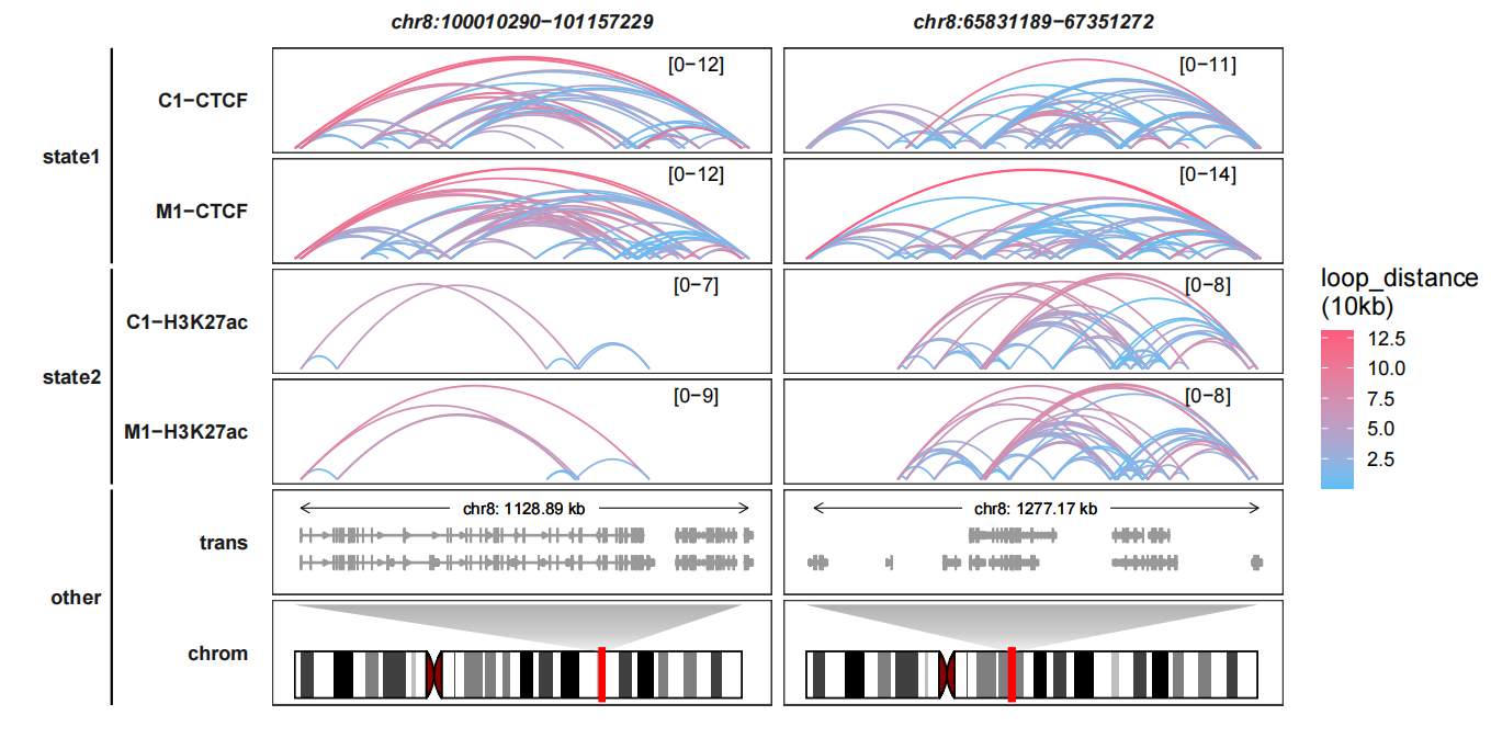
You can just choose suitable style what you like.