3 Align on genome
This chapter we will describe the total ribo-seq workflow with aligning reads on genome. The test dataset is from GSE157519(Adaptive translational pausing is a hallmark of the cellular response to severe environmental stress). You can download raw fastq files to follow this analysis flow.
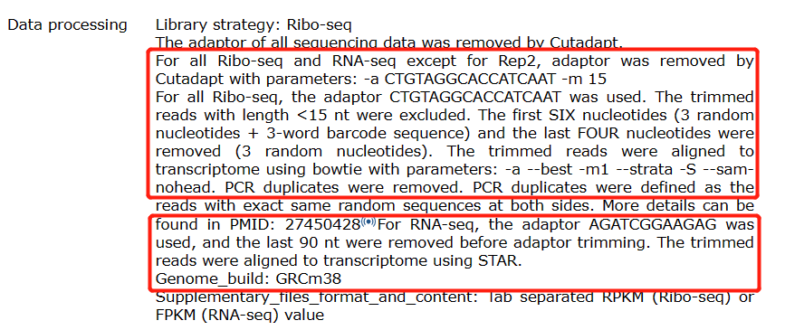
3.1 Check papers data processing
The RNA-seq data was generated using paired-end sequencing, while the Ribo-seq data was generated using single-end sequencing. For convenience, we used the read1 of the RNA-seq data as input for our analysis. The follows are details of paper’s data processing:
3.2 Trim adaptors
Here are the raw fastq files:
library(RiboProfiler)
# ┌────────────────────────────────────────────────────────────────┐
# │                                                                │
# │   Welcome to use RiboProfiler package for Ribo-seq analysis.   │
# │                                                                │
# └────────────────────────────────────────────────────────────────┘
#
# The version of RiboProfiler: 0.0.5
# Any advice or suggestions please contact with me: 3219030654@stu.cpu.edu.cn.

list.files("1.raw-data/","*.gz")
# [1] "SRR12594201.fastq.gz"   "SRR12594205.fastq.gz"   "SRR12594209.fastq.gz"
# [4] "SRR12594210.fastq.gz"   "SRR12594214.fastq.gz"   "SRR12594218.fastq.gz"
# [7] "SRR12594219_1.fastq.gz" "SRR12594223_1.fastq.gz" "SRR12594227_1.fastq.gz"
# [10] "SRR12594228_1.fastq.gz" "SRR12594232_1.fastq.gz" "SRR12594236_1.fastq.gz"
First we trim the adapters for Ribo-seq using batch_adpator_remove function:
dir.create("2.trim-data")

# test function
fq <- list.files(path = "1.raw-data/",pattern = ".gz",full.names = T)

rmd1 <- batch_adpator_remove(fastq_file1 = fq[1:6],
                             output_dir = "2.trim-data/",
                             output_name = paste("tmp_",sapply(strsplit(fq[1:6],split = "\\.|/"), "[",3),
                                                 sep = ""),
                             fastp_params = list(minReadLength = 15,
                                                 adapterSequenceRead1 = "CTGTAGGCACCATCAAT",
                                                 thread = 24))
# ▶ tmp_SRR12594201 has been processed!
# ▶ tmp_SRR12594205 has been processed!
# ▶ tmp_SRR12594209 has been processed!
# ▶ tmp_SRR12594210 has been processed!
# ▶ tmp_SRR12594214 has been processed!
# ▶ tmp_SRR12594218 has been processed!
Then we trim the left and right bases for remaing reads:
# trim bases form left and right
rmd2 <- batch_adpator_remove(fastq_file1 = list.files("2.trim-data/",pattern = ".gz",
                                                      full.names = T),
                             output_dir = "2.trim-data/",
                             output_name = sapply(strsplit(fq[1:6],split = "\\.|/"), "[",3),
                             fastp_params = list(trimFrontRead1 = 6,
                                                 trimTailRead1 = 4,
                                                 adapterTrimming = FALSE,
                                                 thread = 16))

# ▶ SRR12594201 has been processed!
# ▶ SRR12594205 has been processed!
# ▶ SRR12594209 has been processed!
# ▶ SRR12594210 has been processed!
# ▶ SRR12594214 has been processed!
# ▶ SRR12594218 has been processed!

# remove tmp
file.remove(list.files("2.trim-data/",pattern = "^tmp",full.names = T))
Finally we trim adapters for RNA-seq:
# ==============================================================================
# trim rna adapters
# ==============================================================================
rmd3 <- batch_adpator_remove(fastq_file1 = fq[7:12],
                             output_dir = "2.trim-data/",
                             output_name = sapply(strsplit(fq[7:12],split = "\\.|/"), "[",3),
                             fastp_params = list(minReadLength = 15,
                                                 trimFrontRead1 = 1,
                                                 adapterSequenceRead1 = "AGATCGGAAGAG",
                                                 trimTailRead1 = 90,
                                                 thread = 16))

# ▶ SRR12594219_1 has been processed!
# ▶ SRR12594223_1 has been processed!
# ▶ SRR12594227_1 has been processed!
# ▶ SRR12594228_1 has been processed!
# ▶ SRR12594232_1 has been processed!
# ▶ SRR12594236_1 has been processed!
3.3 Build index
3.3.1 Build index for tRNA and rRNA
fetch_trRNA_from_NCBI function can download rRNA and tRNA sequences from NCBI, just supplying with your own species:
# download mouse rRNA and tRNA
fetch_trRNA_from_NCBI(species = "Mus musculus")
# ┌──────────────────────────────────────────────────────────────┐
# │                                                              │
# │   Download tRNA and rRNA sequences from NCBI has finished!   │
# │                                                              │
# └──────────────────────────────────────────────────────────────┘
# ▶ Here are some common species Latin names:
#
#   人类(Homo sapiens), 大鼠(Rattus norvegicus), 小鼠(Mus musculus),
# 斑马鱼(Danio rerio), 红毛猩猩(Pan troglodytes), 家犬(Canis familiaris),
# 草履虫(Dictyostelium discoideum), 猴子(Macaca mulatta), 红松鼠(Tamiasciurus hudsonicus),
# 家兔(Oryctolagus cuniculus), 黄鼠狼(Cricetulus griseus), 南方豹猫(Prionailurus rubiginosus),
# 畜牛(Bos taurus), 绿猴(Chlorocebus sabaeus), 绵羊(Ovis aries),
# 猪(Sus scrofa), 验血鸟(Taeniopygia guttata), 萨摩耶犬(Canis lupus familiaris),
# 膜骨鱼(Takifugu rubripes), 猫(Felis catus), 银狐(Vulpes vulpes),
# 水稻(Oryza sativa), 吸血蝙蝠(Desmodus rotundus), 巴西三带蚊(Aedes aegypti),
# 印度大象(Elephas maximus), 狼(Canis lupus), 仓鼠(Cricetulus griseus),
# 刺参(Strongylocentrotus purpuratus), 山羊(Capra hircus), 兔子(Oryctolagus cuniculus),
# 黄猴(Macaca fascicularis), 石斑鱼(Epinephelus coioides), 柴犬(Canis lupus familiaris),
# 蚯蚓(Eisenia fetida), 小萤火虫(Luciola cruciata), 白化病毒(White spot syndrome virus),
# 河北地蜂(Apis cerana), 喜马拉雅兔(Ochotona curzoniae), 裸鼠(Heterocephalus glaber),
# 马(Equus caballus), 胡萝卜野生种(Daucus carota subsp. carota), 水牛(Bubalus bubalis),
# 歌鸲(Erithacus rubecula), 美国黑熊(Ursus americanus), 鲨鱼(Callorhinchus milii),
# 大黄蜂(Vespa mandarinia), 蜡螟(Galleria mellonella), 黄斑蝶(Papilio xuthus),
# 皇家企鹅(Aptenodytes forsteri), 银河野猪(Sus scrofa)
We can check the sequence:
system("head Mus_musculus_trRNA.fa")
# >NR_003278.3 Mus musculus 18S ribosomal RNA (Rn18s), ribosomal RNA
# ACCTGGTTGATCCTGCCAGGTAGCATATGCTTGTCTCAAAGATTAAGCCATGCATGTCTAAGTACGCACGGCCGGTACAG
# TGAAACTGCGAATGGCTCATTAAATCAGTTATGGTTCCTTTGGTCGCTCGCTCCTCTCCTACTTGGATAACTGTGGTAAT
# TCTAGAGCTAATACATGCCGACGGGCGCTGACCCCCCTTCCCGGGGGGGGATGCGTGCATTTATCAGATCAAAACCAACC
# CGGTGAGCTCCCTCCCGGCTCCGGCCGGGGGTCGGGCGCCGGCGGCTTGGTGACTCTAGATAACCTCGGGCCGATCGCAC
# GCCCCCCGTGGCGGCGACGACCCATTCGAACGTCTGCCCTATCAACTTTCGATGGTAGTCGCCGTGCCTACCATGGTGAC
# CACGGGTGACGGGGAATCAGGGTTCGATTCCGGAGAGGGAGCCTGAGAAACGGCTACCACATCCAAGGAAGGCAGCAGGC
# GCGCAAATTACCCACTCCCGACCCGGGGAGGTAGTGACGAAAAATAACAATACAGGACTCTTTCGAGGCCCTGTAATTGG
# AATGAGTCCACTTTAAATCCTTTAACGAGGATCCATTGGAGGGCAAGTCTGGTGCCAGCAGCCGCGGTAATTCCAGCTCC
# AATAGCGTATATTAAAGTTGCTGCAGTTAAAAAGCTCGTAGTTGGATCTTGGGAGCGGGCGGGCGGTCCGCCGCGAGGCG
# [1] 0
trRNA_index_build is used to build index based on bowtie2 software:
# buid index for tRNA and tRNA
trRNA_index_build(trRNA_file = "Mus_musculus_trRNA.fa",
                  prefix = "GRCm38_trRNA")
# ┌────────────────────────────────────────────────────┐
# │                                                    │
# │   Building index for tRNA and rRNA has finished!   │
# │                                                    │
# └────────────────────────────────────────────────────┘
3.3.2 Build index for genome
Genome sequence can be downloaded from some database like ensembl, UCSC, gencode. Here we use mouse GRCm38 genome sequence from ensembl. reference_index_build is used to build index based on Rhisat2 software:
reference_index_build(reference_file = "Mus_musculus.GRCm38.dna.primary_assembly.fa",
                      prefix = "GRCm38_ref",
                      threads = 8)
# ┌────────────────────────────────────────────────────┐
# │                                                    │
# │   Building index for reference has finished!       │
# │                                                    │
# └────────────────────────────────────────────────────┘
3.4 Check index files
The index files have been save in 0.index-data/ directory:
list.files("0.index-data/",recursive = T)
# [1] "ref-index/GRCm38_ref.1.ht2"         "ref-index/GRCm38_ref.2.ht2"
# [3] "ref-index/GRCm38_ref.3.ht2"         "ref-index/GRCm38_ref.4.ht2"
# [5] "ref-index/GRCm38_ref.5.ht2"         "ref-index/GRCm38_ref.6.ht2"
# [7] "ref-index/GRCm38_ref.7.ht2"         "ref-index/GRCm38_ref.8.ht2"
# [9] "rtRNA-index/GRCm38_trRNA.1.bt2"     "rtRNA-index/GRCm38_trRNA.2.bt2"
# [11] "rtRNA-index/GRCm38_trRNA.3.bt2"     "rtRNA-index/GRCm38_trRNA.4.bt2"
# [13] "rtRNA-index/GRCm38_trRNA.rev.1.bt2" "rtRNA-index/GRCm38_trRNA.rev.2.bt2"
3.5 Remove rRNA and tRNA contamination
The RNA content in a prokaryotic or an eukaryotic cell consists of 80–90% rRNA, 10–15% transfer RNA (tRNA) and 3–7% messenger RNA (mRNA) and regulatory ncRNA.The presence of abundant rRNA can introduce substantial bias to transcriptome data. A number of protein coding genes contain some rRNA-like sequence segments, so their expression levels can be strongly overestimated unless the rRNA reads are removed. Furthermore, rRNA removal can greatly reduce the data size for downstream analysis and accelerate the entire workflow. Here we align the reads on tRNA and rRNA sequences to remove reads which come from tRNA and rRNA.
bowtie2_align will try download windows executable bowtie2 software from bowtie2. You can download it by yourself if this failed. Making sure the software is in parent directory:
list.files("bowtie2-2.5.1-mingw-x86_64/",full.names = T) |>
  head()
# [1] "bowtie2-2.5.1-mingw-x86_64/AUTHORS"
# [2] "bowtie2-2.5.1-mingw-x86_64/bowtie2"
# [3] "bowtie2-2.5.1-mingw-x86_64/bowtie2-align-l"
# [4] "bowtie2-2.5.1-mingw-x86_64/bowtie2-align-l-debug"
# [5] "bowtie2-2.5.1-mingw-x86_64/bowtie2-align-s"
# [6] "bowtie2-2.5.1-mingw-x86_64/bowtie2-align-s-debug"
Now remove the tRNA and rRNA sequences using bowtie2:
# ==============================================================================
# remove trRNA sequence
# ==============================================================================
dir.create("3.rmtrRNA-data")
# loop for remove trRNA sequence
clean_fq <- list.files("2.trim-data/",pattern = ".fastq.gz",full.names = T)
clean_fq
# [1] "2.trim-data/SRR12594201_R1.fastq.gz"   "2.trim-data/SRR12594205_R1.fastq.gz"
# [3] "2.trim-data/SRR12594209_R1.fastq.gz"   "2.trim-data/SRR12594210_R1.fastq.gz"
# [5] "2.trim-data/SRR12594214_R1.fastq.gz"   "2.trim-data/SRR12594218_R1.fastq.gz"
# [7] "2.trim-data/SRR12594219_1_R1.fastq.gz" "2.trim-data/SRR12594223_1_R1.fastq.gz"
# [9] "2.trim-data/SRR12594227_1_R1.fastq.gz" "2.trim-data/SRR12594228_1_R1.fastq.gz"
# [11] "2.trim-data/SRR12594232_1_R1.fastq.gz" "2.trim-data/SRR12594236_1_R1.fastq.gz"
output_sam <- paste("3.rmtrRNA-data/",sapply(strsplit(clean_fq,split = "\\.|/"), "[",3),
                    ".sam",sep = "")
output_sam
# [1] "3.rmtrRNA-data/SRR12594201_R1.sam"   "3.rmtrRNA-data/SRR12594205_R1.sam"
# [3] "3.rmtrRNA-data/SRR12594209_R1.sam"   "3.rmtrRNA-data/SRR12594210_R1.sam"
# [5] "3.rmtrRNA-data/SRR12594214_R1.sam"   "3.rmtrRNA-data/SRR12594218_R1.sam"
# [7] "3.rmtrRNA-data/SRR12594219_1_R1.sam" "3.rmtrRNA-data/SRR12594223_1_R1.sam"
# [9] "3.rmtrRNA-data/SRR12594227_1_R1.sam" "3.rmtrRNA-data/SRR12594228_1_R1.sam"
# [11] "3.rmtrRNA-data/SRR12594232_1_R1.sam" "3.rmtrRNA-data/SRR12594236_1_R1.sam"
rm_trRNAfq <- paste("3.rmtrRNA-data/",sapply(strsplit(clean_fq,split = "\\.|/"), "[",3),
                    "_rmtrRNA.fq",sep = "")
# [1] "3.rmtrRNA-data/SRR12594201_R1_rmtrRNA.fq"   "3.rmtrRNA-data/SRR12594205_R1_rmtrRNA.fq"
# [3] "3.rmtrRNA-data/SRR12594209_R1_rmtrRNA.fq"   "3.rmtrRNA-data/SRR12594210_R1_rmtrRNA.fq"
# [5] "3.rmtrRNA-data/SRR12594214_R1_rmtrRNA.fq"   "3.rmtrRNA-data/SRR12594218_R1_rmtrRNA.fq"
# [7] "3.rmtrRNA-data/SRR12594219_1_R1_rmtrRNA.fq" "3.rmtrRNA-data/SRR12594223_1_R1_rmtrRNA.fq"
# [9] "3.rmtrRNA-data/SRR12594227_1_R1_rmtrRNA.fq" "3.rmtrRNA-data/SRR12594228_1_R1_rmtrRNA.fq"
# [11] "3.rmtrRNA-data/SRR12594232_1_R1_rmtrRNA.fq" "3.rmtrRNA-data/SRR12594236_1_R1_rmtrRNA.fq"

# batch align
lapply(seq_along(clean_fq),function(x){
  bowtie2_align(index = "0.index-data/rtRNA-index/GRCm38_trRNA",
                fq_file1 = clean_fq[x],
                output_file = output_sam[x],
                threads = 24,
                bowtie2_params = paste("--un ",rm_trRNAfq[x],sep = ""))
}) -> tmp

# ▶ 3.rmtrRNA-data/SRR12594201_R1.sam has been processed!
# ▶ 3.rmtrRNA-data/SRR12594205_R1.sam has been processed!
# ▶ 3.rmtrRNA-data/SRR12594209_R1.sam has been processed!
# ...

# remove tmp sam
file.remove(list.files("3.rmtrRNA-data/",pattern = ".sam$",full.names = T))
3.5.1 mapping info visualization
plot_mapinfo allows you plot the details of mapping:
# plot
map_info <- list.files("3.rmtrRNA-data/",pattern = "mapinfo.txt",full.names = TRUE)

# barplot
plot_mapinfo(mapinfo_file = map_info,
             file_name = sapply(strsplit(clean_fq,split = "\\.|/|_"), "[",3))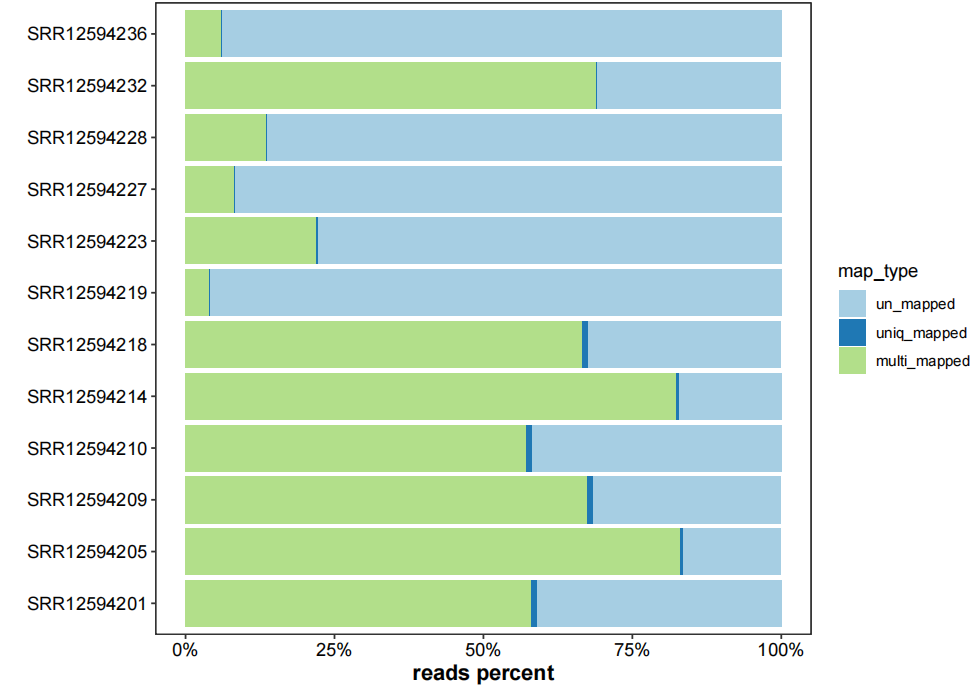
Or plot a table:
# table
plot_mapinfo(mapinfo_file = map_info,
             file_name = sapply(strsplit(clean_fq,split = "\\.|/|_"), "[",3),
             plot_type = "table")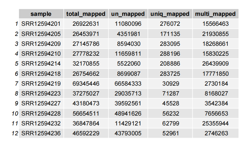
3.6 Map to genome
batch_hisat_align uses Rhisat2 to align reads on genome:
# ==============================================================================
# map to genome
# ==============================================================================
dir.create("4.map-data")

# batch map to genome
fq_file1 <- list.files("3.rmtrRNA-data/",pattern = ".fq$",full.names = T)
output_file <- c("ribo_nromal_rep1","ribo_700_2h_rep1","ribo_700_2h_r2h_rep1",
                 "ribo_nromal_rep2","ribo_700_2h_rep2","ribo_700_2h_r2h_rep2",
                 "rna_nromal_rep1","rna_700_2h_rep1","rna_700_2h_r2h_rep1",
                 "rna_nromal_rep2","rna_700_2h_rep2","rna_700_2h_r2h_rep2")

batch_hisat_align(index = "0.index-data/ref-index/GRCm38_ref",
                  fq_file1 = fq_file1,
                  output_dir = "4.map-data/",
                  output_file = output_file,
                  threads = 24,hisat2_params = list(k = 1))

# ▶ ribo_nromal_rep1 has been processed!
# ▶ ribo_700_2h_rep1 has been processed!
# ▶ ribo_700_2h_r2h_rep1 has been processed!
# ...
Plot mapinfo barplot:
map_info_geome <- list.files("4.map-data/",pattern = "mapinfo.txt",full.names = TRUE)

# barplot
plot_mapinfo(mapinfo_file = map_info_geome,
             file_name = sapply(strsplit(map_info_geome,split = "_mapinfo.txt|/"), "[",2))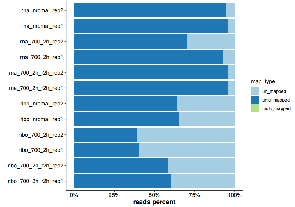
Plot with a table:
# table
plot_mapinfo(mapinfo_file = map_info_geome,
             file_name = sapply(strsplit(map_info_geome,split = "_mapinfo.txt|/"), "[",2),
             plot_type = "table")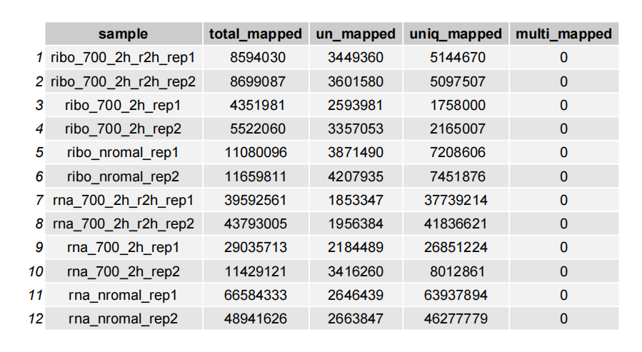
3.7 Sam to bam
Covert the sam files into bam format:
# ==============================================================================
# sam to bam
# ==============================================================================
dir.create("4.map-data/bam-data",recursive = TRUE)

# convert sam to bam
batch_sam2bam(sam_file = paste("4.map-data/",output_file,".sam",sep = ""),
              bam_file = paste("4.map-data/bam-data/",output_file,sep = ""))

# [bam_sort_core] merging from 3 files and 1 in-memory blocks...
# ▶ 4.map-data/ribo_nromal_rep1.sam has been processed!
#   [bam_sort_core] merging from 1 files and 1 in-memory blocks...
# ▶ 4.map-data/ribo_700_2h_rep1.sam has been processed!
#   [bam_sort_core] merging from 2 files and 1 in-memory blocks...
# ▶ 4.map-data/ribo_700_2h_r2h_rep1.sam has been processed!
#   [bam_sort_core] merging from 3 files and 1 in-memory blocks...
# ...
3.8 Ribo-seq QC check
3.8.1 prepare longest transcript
First we should prepare the longest transcript for each protein gene with gene annotation file:
dir.create("5.analysis-data")

setwd("5.analysis-data")
# ==============================================================================
# 1_prepare gene annotation file
# ==============================================================================
pre_longest_trans_info(gtf_file = "../Mus_musculus.GRCm38.102.gtf.gz",
                       out_file = "longest_info.txt")
# ================================ job finished.
3.8.2 prepare QC data
pre_qc_data will produce QC data for ribo-seq sam files:
# ==============================================================================
# 2_prepare Ribo QC data
# ==============================================================================
sam_file = list.files("../4.map-data/",pattern = "^ribo.*sam$",full.names = TRUE)
sam_file
# [1] "../4.map-data/ribo_700_2h_r2h_rep1.sam" "../4.map-data/ribo_700_2h_r2h_rep2.sam"
# [3] "../4.map-data/ribo_700_2h_rep1.sam"     "../4.map-data/ribo_700_2h_rep2.sam"
# [5] "../4.map-data/ribo_nromal_rep1.sam"     "../4.map-data/ribo_nromal_rep2.sam"

sample_name <- sapply(strsplit(list.files("../4.map-data/",pattern = "^ribo.*sam$"),
                               split = ".sam"), "[",1)
sample_name
# [1] "ribo_700_2h_r2h_rep1" "ribo_700_2h_r2h_rep2" "ribo_700_2h_rep1"
# [4] "ribo_700_2h_rep2"     "ribo_nromal_rep1"     "ribo_nromal_rep2"

# run
pre_qc_data(longest_trans_file = "longest_info.txt",
            sam_file = sam_file,
            out_file = paste(sample_name,".qc.txt",sep = ""),
            mapping_type = "genome",
            seq_type = "singleEnd")
# "Transforming genomic positions into transcriptome positions has been done successfully."
#
# "Processing sam files..."
#
# "../4.map-data/ribo_700_2h_r2h_rep1.sam has been processed."
#
# "../4.map-data/ribo_700_2h_r2h_rep2.sam has been processed."
#
# "../4.map-data/ribo_700_2h_rep1.sam has been processed."
# ...
3.8.3 load qc data
load_qc_data will read all the qc data into R and return a data frame:
# load qc data
qc_df <- load_qc_data()

# QC input files:
# ribo_700_2h_r2h_rep1.qc.txt
# ribo_700_2h_r2h_rep2.qc.txt
# ribo_700_2h_rep1.qc.txt
# ribo_700_2h_rep2.qc.txt
# ribo_nromal_rep1.qc.txt
# ribo_nromal_rep2.qc.txt

# check
head(qc_df,3)
#   length framest relst framesp relsp feature counts               sample group
# 1     30       2  1988       1  -118       3      1 ribo_700_2h_r2h_rep1    NA
# 2     28       1   988       2 -2060       3      1 ribo_700_2h_r2h_rep1    NA
# 3     25       1  1042       2  -374       3      1 ribo_700_2h_r2h_rep1    NA

qc_df$length <- factor(qc_df$length)
qc_df$sample <- factor(qc_df$sample,
                       levels = c("ribo_nromal_rep1","ribo_700_2h_rep1","ribo_700_2h_r2h_rep1",
                                  "ribo_nromal_rep2","ribo_700_2h_rep2","ribo_700_2h_r2h_rep2")
                       )
3.8.4 qc visualization
Now plot the qc data with multiple kinds of graph, first check the length distribution of fragments:
# length distribution
qc_plot(qc_data = qc_df,type = "length",facet_wrap_list = list(ncol = 3))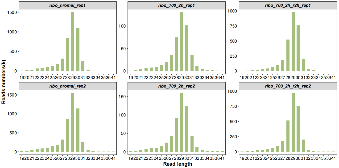
Frames with length distribution:
# length with frame
qc_plot(qc_data = qc_df,type = "length_frame",facet_wrap_list = list(ncol = 3))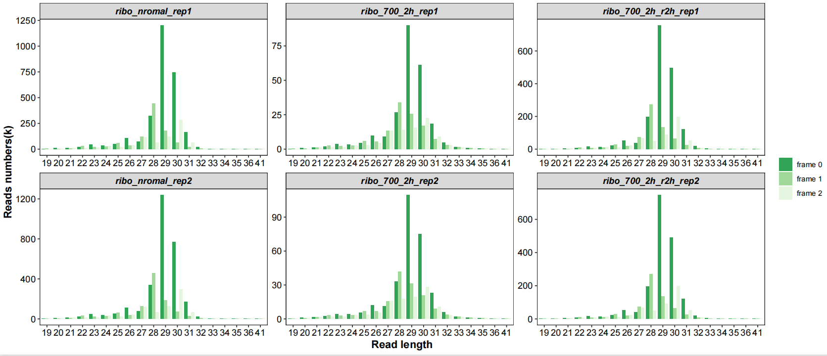
Different region features:
# region features
qc_plot(qc_data = qc_df,type = "feature",facet_wrap_list = list(ncol = 3))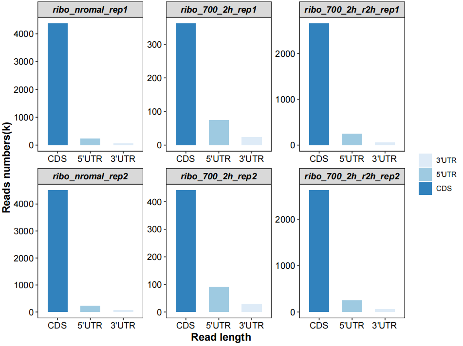
All frames ratio:
# all frames
qc_plot(qc_data = qc_df,type = "frame",facet_wrap_list = list(ncol = 3))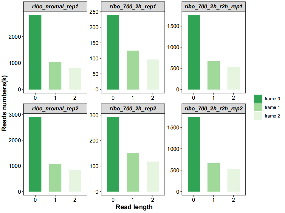
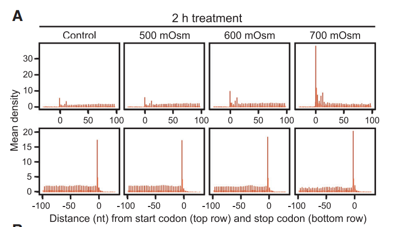
Realtive to start codon with periodicity:
# relative to start/stop site 5x10
rel_to_start_stop(qc_data = qc_df,type = "relst",
                  facet_wrap_list = list(ncol = 3,scales = "fixed"))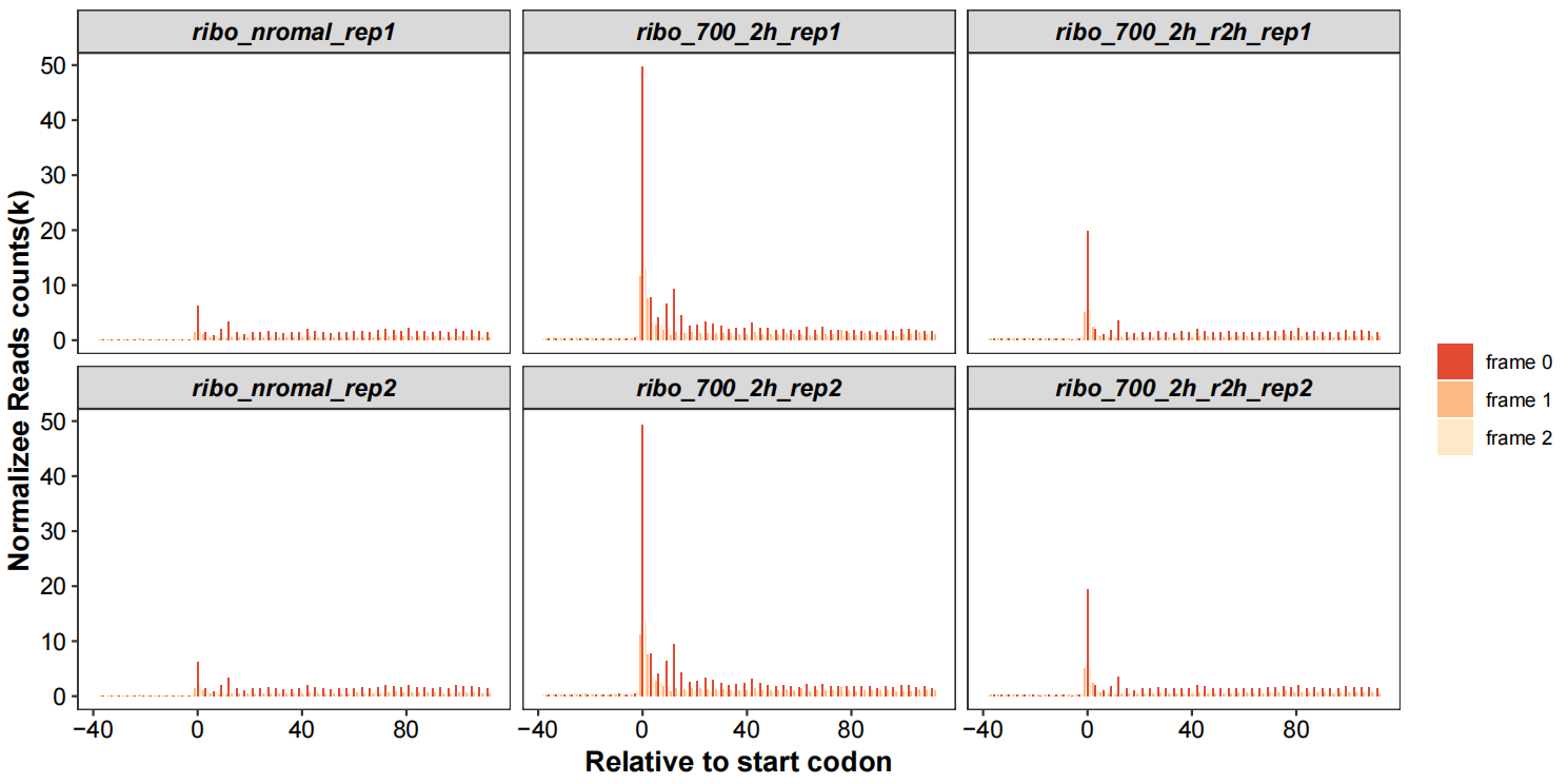
You can zoom the distance:
rel_to_start_stop(qc_data = qc_df,type = "relst",
                  dist_range = c(-20,60),
                  facet_wrap_list = list(ncol = 3,scales = "fixed"))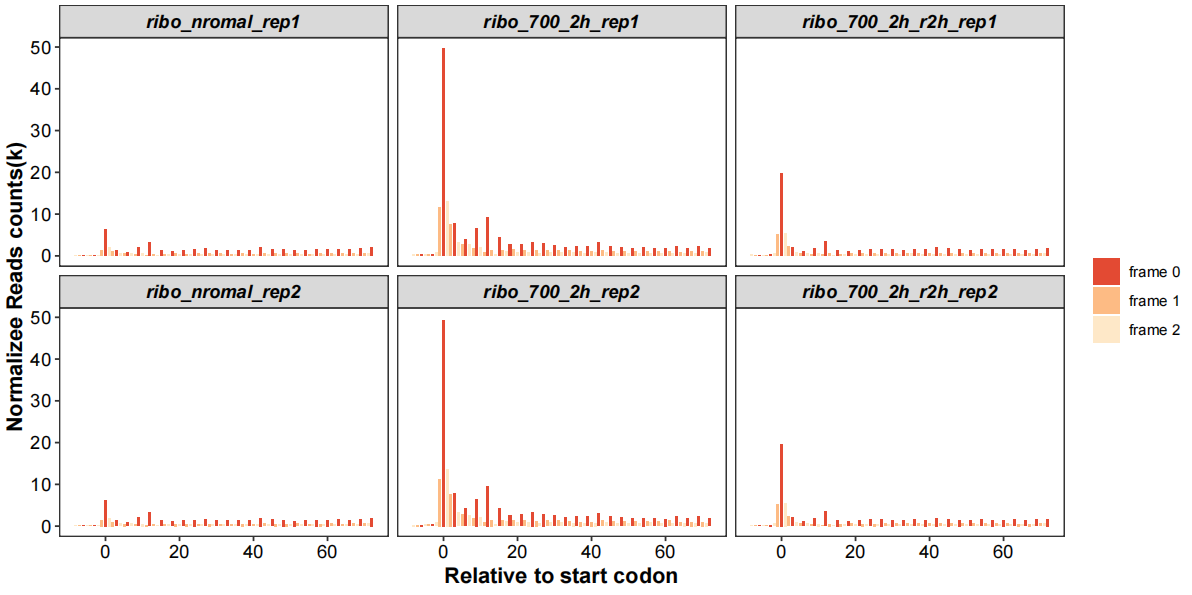
Realtive to stop codon with periodicity:
rel_to_start_stop(qc_data = qc_df,type = "relsp",
                  facet_wrap_list = list(ncol = 3,scales = "fixed"))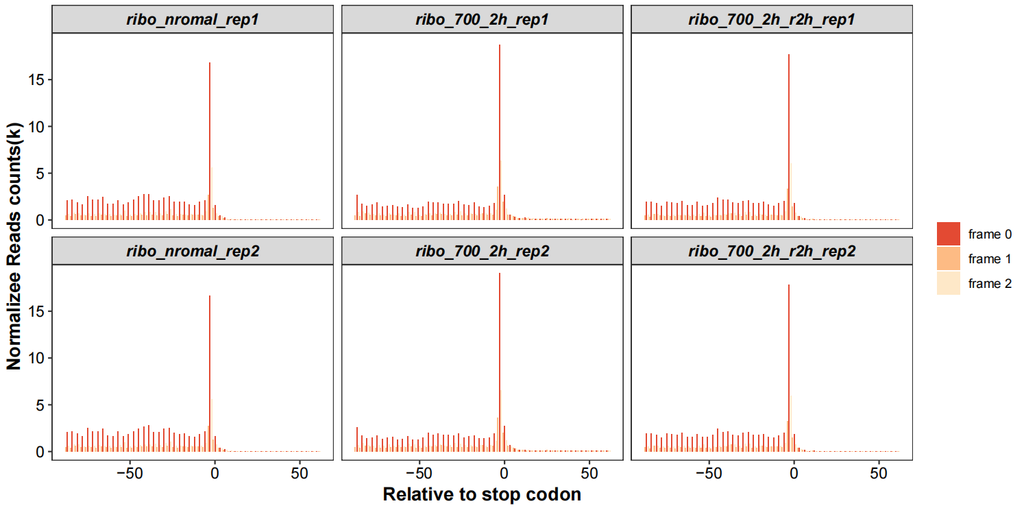
Here is the origin paper’s figure:
3.10 Calculate Ribo density and RNA coverage
This step will produce each ribosome density and RNA coverage on genomic positions:
# ==============================================================================
# 3_prepare Ribo density and RNA coverage data
# ==============================================================================
# calculate Ribo density
pre_ribo_density_data(sam_file = sam_file,
                      out_file = paste(sample_name,".density.txt",sep = ""))

# ../4.map-data/ribo_700_2h_r2h_rep1.sam has been processed!
# ../4.map-data/ribo_700_2h_r2h_rep2.sam has been processed!
# ../4.map-data/ribo_700_2h_rep1.sam has been processed!
# ../4.map-data/ribo_700_2h_rep2.sam has been processed!
# ../4.map-data/ribo_nromal_rep1.sam has been processed!
# ../4.map-data/ribo_nromal_rep2.sam has been processed!
# NULL

# calculate RNA coverage
bam_file_rna = list.files("../4.map-data/bam-data/",pattern = "^rna.*bam$",full.names = TRUE)
bam_file_rna
# [1] "../4.map-data/bam-data/rna_700_2h_r2h_rep1.bam" "../4.map-data/bam-data/rna_700_2h_r2h_rep2.bam"
# [3] "../4.map-data/bam-data/rna_700_2h_rep1.bam"     "../4.map-data/bam-data/rna_700_2h_rep2.bam"
# [5] "../4.map-data/bam-data/rna_nromal_rep1.bam"     "../4.map-data/bam-data/rna_nromal_rep2.bam"

sample_name_rna <- sapply(strsplit(list.files("../4.map-data/bam-data/",pattern = "^rna.*bam$"),
                               split = ".bam"), "[",1)
sample_name_rna
# [1] "rna_700_2h_r2h_rep1" "rna_700_2h_r2h_rep2" "rna_700_2h_rep1"     "rna_700_2h_rep2"
# [5] "rna_nromal_rep1"     "rna_nromal_rep2"

pre_rna_coverage_data(bam_file = bam_file_rna,
                      out_file = paste(sample_name_rna,".coverage.txt",sep = ""))

# ../4.map-data/bam-data/rna_700_2h_r2h_rep1.bam has been processed!
# ../4.map-data/bam-data/rna_700_2h_r2h_rep2.bam has been processed!
# ../4.map-data/bam-data/rna_700_2h_rep1.bam has been processed!
# ../4.map-data/bam-data/rna_700_2h_rep2.bam has been processed!
# ../4.map-data/bam-data/rna_nromal_rep1.bam has been processed!
# ../4.map-data/bam-data/rna_nromal_rep2.bam has been processed!
3.11 Coordinate transformation
Now we need to transform the genomic coordinates into transcriptomic coordinates according to the longest transcript file prepared before:
# ==============================================================================
# 4_transform genomic coordinate into transcriotomic coordinate
# ==============================================================================
pre_gene_trans_density(gene_anno = "longest_info.txt",
                       density_file = c(paste(sample_name,".density.txt",sep = ""),
                                        paste(sample_name_rna,".coverage.txt",sep = "")),
                       out_file = c(paste(sample_name,".trans.txt",sep = ""),
                                    paste(sample_name_rna,".trans.txt",sep = "")))

# 2.density-data/ribo_700_2h_r2h_rep1.density.txt  has been processed!
# 2.density-data/ribo_700_2h_r2h_rep2.density.txt  has been processed!
# ...
3.12 Track plot
Once if we have ribo density and RNA coverage files, we can use load_track_data to load the data and track_plot to visualize data:
3.12.1 load track data
# ==============================================================================
# 5_load denisty and coverage data for specific gene
# ==============================================================================
track_df <- load_track_data(ribo_file = paste(sample_name,".trans.txt",sep = ""),
                            rna_file = paste(sample_name_rna,".trans.txt",sep = ""),
                            sample_name = paste(rep(c("700_2h_r2h","700_2h","normal"),each = 2),
                                                c("_rep1","_rep2"),sep = ""),
                            gene_list = c("Ndufb3","Ndufb6","Rps7","Uqcrfs1","Ndufv1","Sat1"))

# check
head(track_df,3)
#   gene_name           trans_id transpos density type     sample
# 1    Ndufb3 ENSMUST00000027193        1       0 ribo 700_2h_r2h
# 2    Ndufb3 ENSMUST00000027193        2       0 ribo 700_2h_r2h
# 3    Ndufb3 ENSMUST00000027193        3       0 ribo 700_2h_r2h
3.12.2 plot tracks
# 6x12
track_plot(signal_data = track_df,
           gene_anno = "longest_info.txt",
           sample_order = c("normal_rep1","normal_rep2","700_2h_rep1","700_2h_rep2",
                            "700_2h_r2h_rep1","700_2h_r2h_rep2"),
           remove_trans_panel_border = T,
           range_pos = c(0.75,0.1))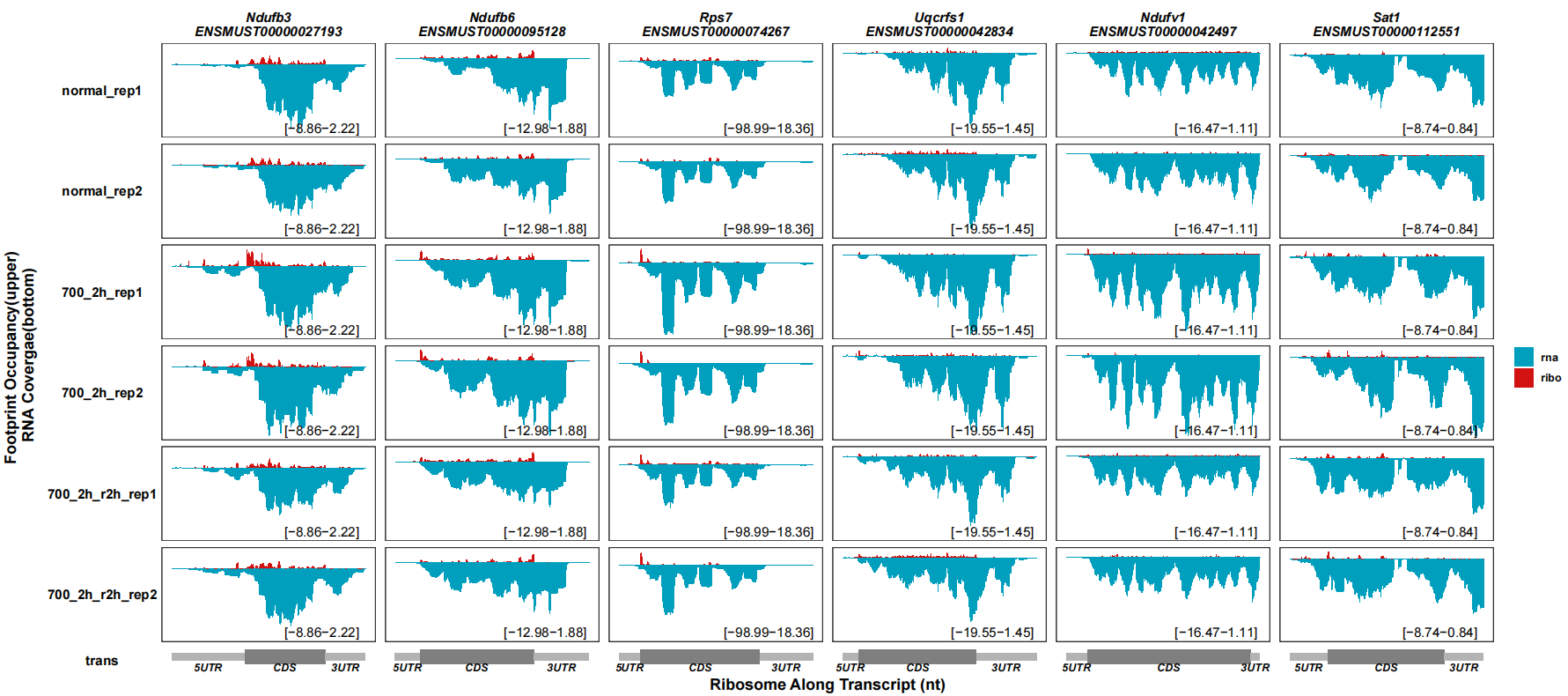
You can not reverse the RNA coverage track:
track_plot(signal_data = track_df,
           gene_anno = "longest_info.txt",
           sample_order = c("normal_rep1","normal_rep2","700_2h_rep1","700_2h_rep2",
                            "700_2h_r2h_rep1","700_2h_r2h_rep2"),
           remove_trans_panel_border = T,
           reverse_rna = F,
           signal_col = c("ribo" = "red","rna" = "grey80"))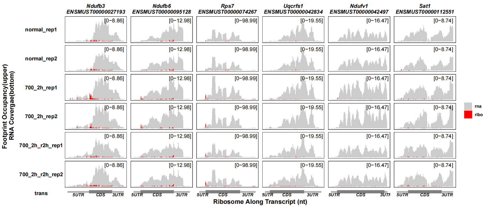
Sometimes the range of RNA coverage is much than ribo density, you can use rna_signal_scale the rescale the RNA coverage range:
track_plot(signal_data = track_df,
           gene_anno = "longest_info.txt",
           sample_order = c("normal_rep1","normal_rep2","700_2h_rep1","700_2h_rep2",
                            "700_2h_r2h_rep1","700_2h_r2h_rep2"),
           remove_trans_panel_border = T,
           reverse_rna = F,
           signal_col = c("ribo" = "red","rna" = "grey80"),
           rna_signal_scale = 0.1)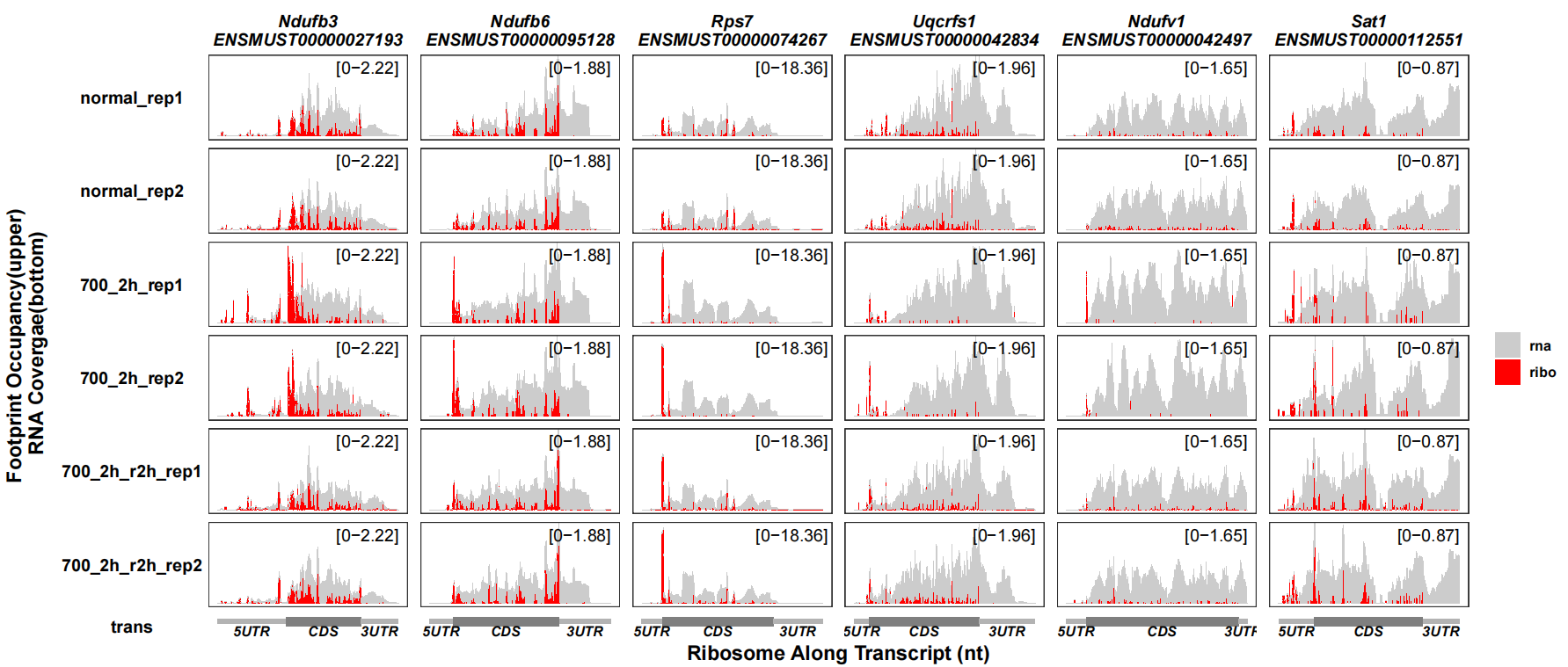
The reversed RNA track with rescaled coverage:
track_plot(signal_data = track_df,
           gene_anno = "longest_info.txt",
           sample_order = c("normal_rep1","normal_rep2","700_2h_rep1","700_2h_rep2",
                            "700_2h_r2h_rep1","700_2h_r2h_rep2"),
           remove_trans_panel_border = T,
           signal_col = c("ribo" = "red","rna" = "grey80"),
           rna_signal_scale = 0.1)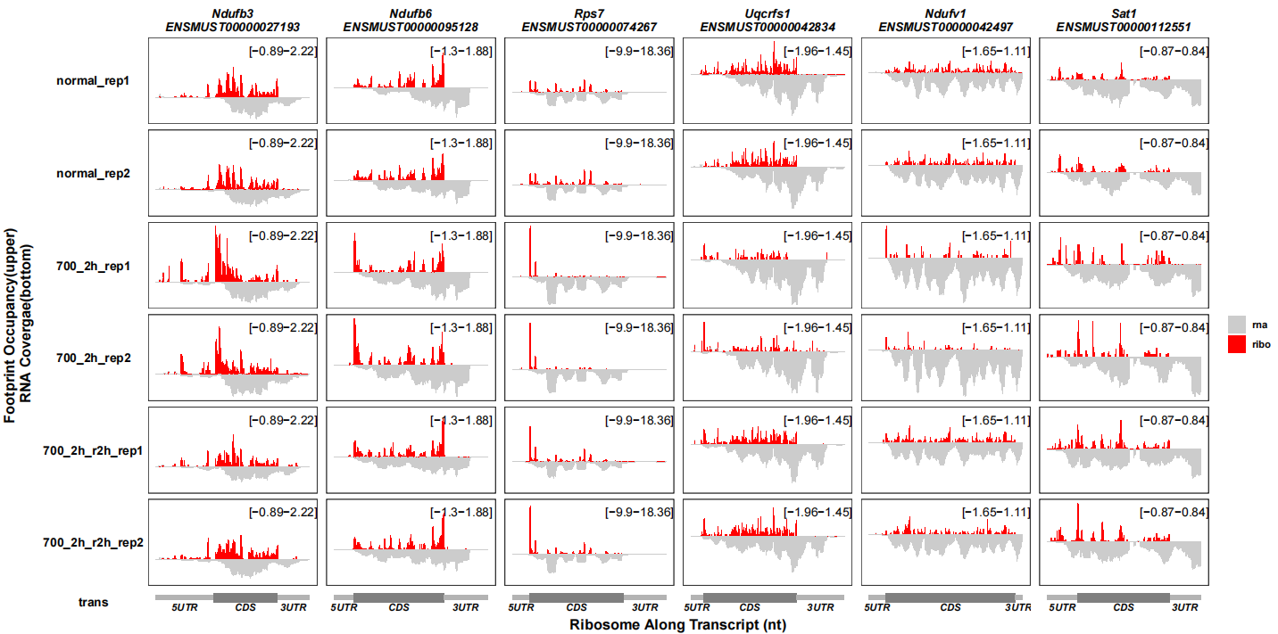
show_ribo_only can be setted to show only ribo tracks:
track_plot(signal_data = track_df,
           gene_anno = "longest_info.txt",
           sample_order = c("normal_rep1","normal_rep2","700_2h_rep1","700_2h_rep2",
                            "700_2h_r2h_rep1","700_2h_r2h_rep2"),
           remove_trans_panel_border = T,
           show_ribo_only = T)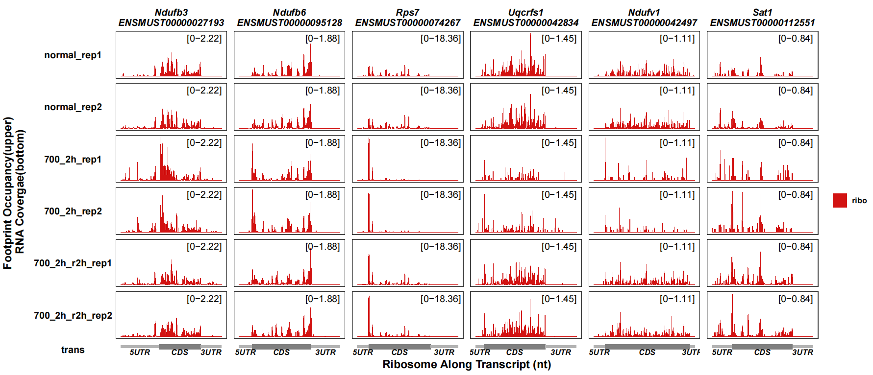
3.13 Quantification
You can use Rsubread featureCounts function to get count matrix:
library(Rsubread)

exp <- featureCounts(files = list.files("../4.map-data/bam-data/",pattern = ".bam$",full.names = T),
                     annot.ext = "../Mus_musculus.GRCm38.102.gtf.gz",
                     isGTFAnnotationFile = T,
                     GTF.featureType = "exon",
                     GTF.attrType = "gene_id",
                     GTF.attrType.extra = c("gene_name","gene_biotype"),
                     isPairedEnd = FALSE,
                     nthreads = 12)

counts <- exp$counts
head(counts[1:3,1:3])
#                    ribo_700_2h_r2h_rep1.bam ribo_700_2h_r2h_rep2.bam ribo_700_2h_rep1.bam
# ENSMUSG00000102693                        0                        0                    0
# ENSMUSG00000064842                        0                        2                    0
# ENSMUSG00000051951                        0                        0                    0

tpm <- count_to_tpm(fc_obj = exp)
head(tpm[1:3,1:3])
#              gene_id ribo_700_2h_r2h_rep1.bam ribo_700_2h_r2h_rep2.bam
# 1 ENSMUSG00000000001                 35.70944                 35.37493
# 2 ENSMUSG00000000003                  0.00000                  0.00000
# 3 ENSMUSG00000000028                 11.93136                 11.52324
You can do other related analysis with other tools based on these matrix data.