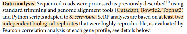
6 SeRP data analysis
6.1 Introduction
We show a entire example to analysis SeRP data which from Cotranslational assembly of protein complexes in eukaryotes revealed by ribosome profiling and the related GSE number is GSE116570. You can download the raw fastq files through other ways.
Here shows the simple data processing describtion:
6.2 Extract yeast longest transcript sequence
Condidering most transcripts have no UTRs(untranslated regions) of Saccharomyces cerevisiae.So we extend 50 bases upstream and downstream for each transcript. We choose to map the reads on transcriptome. Now we use BioSeqUtils to extract fasta:
library(BioSeqUtils)
library(RiboProfiler)

# ==============================================================================
# get longest transcript
# ==============================================================================
# make object
mytest <- loadGenomeGTF(gtfPath = "Saccharomyces_cerevisiae.R64-1-1.105.gtf",
                        genomePath = "Saccharomyces_cerevisiae.R64-1-1.dna.toplevel.fa",
                        filterProtein = T)
## GenomeGTF object for Extracting sequences.
## GTF file is loaded.
## genome file is loaded.
## representTrans file is NULL.
## intron slot is NULL.

# select all genes
gene <- unique(mytest@gtf$gene_name)

# return all transcript info
all <- getTransInfo(object = mytest,geneName = gene,selecType = "lcds",topN = 1)

# extend sequence
extend <- getFeatureFromGenome(mytest,geneName = all$gene_name,
                               type = "exon",
                               up.extend = 50,
                               dn.extend = 50)

# output
Biostrings::writeXStringSet(extend,filepath = "sac_longest_trans.fa",format = "fasta")

# check
system("head sac_longest_trans.fa")
# >AAC1|YMR056C|YMR056C_mRNA|51|978|1030|CD
# CAGATTCTCGTATCTGTTATTCTTTTCTATTTTTCCTTTTTACAGCAGTAATGTCTCACACAGAAACACAGACTCAGCAG
# TCACACTTCGGTGTGGACTTCCTTATGGGCGGCGTTTCTGCTGCCATTGCGAAGACGGGTGCCGCTCCCATTGAACGGGT
# GAAACTGTTGATGCAGAATCAAGAAGAGATGCTTAAACAGGGCTCGTTGGATACACGGTACAAGGGAATTTTAGATTGCT
# TCAAGAGGACTGCGACTCATGAAGGTATTGTGTCGTTCTGGAGGGGTAACACCGCCAATGTTCTCCGGTATTTCCCCACG
# CAGGCGCTGAATTTTGCCTTCAAAGACAAAATTAAGTCGTTGTTGAGTTACGACAGAGAGCGCGATGGGTATGCCAAGTG
# GTTTGCTGGAAATCTTTTCTCTGGTGGAGCGGCTGGTGGTTTGTCGCTTCTATTTGTATATTCCTTGGACTACGCAAGGA
# CGCGGCTTGCAGCGGATGCTAGGGGTTCTAAGTCAACCTCGCAAAGACAGTTTAATGGATTGCTAGACGTGTATAAGAAG
# ACACTGAAAACGGACGGGTTGTTGGGTCTGTACCGTGGGTTTGTGCCCTCAGTTCTGGGTATCATTGTCTACAGAGGTCT
# GTACTTTGGCTTGTACGATTCTTTCAAGCCTGTGCTGTTGACGGGGGCTCTAGAGGGGTCCTTTGTTGCCTCTTTCCTAT
# [1] 0
6.3 Build index for tRNA, rRNA and reference
# ==============================================================================
# build index
# ==============================================================================

# download mouse rRNA and tRNA
fetch_trRNA_from_NCBI(species = "Saccharomyces cerevisiae")
# ┌──────────────────────────────────────────────────────────────┐
# │                                                              │
# │   Download tRNA and rRNA sequences from NCBI has finished!   │
# │                                                              │
# └──────────────────────────────────────────────────────────────┘

# build index
trRNA_index_build(trRNA_file = "Saccharomyces_cerevisiae_trRNA.fa",
                  prefix = "sac_trRNA")
# ┌────────────────────────────────────────────────────┐
# │                                                    │
# │   Building index for tRNA and rRNA has finished!   │
# │                                                    │
# └────────────────────────────────────────────────────┘

reference_index_build(reference_file = "sac_longest_trans.fa",
                      prefix = "sac_ref",
                      threads = 24)
# ┌────────────────────────────────────────────────┐
# │                                                │
# │   Building index for reference has finished!   │
# │                                                │
# └────────────────────────────────────────────────┘
6.4 Trim adapters for raw fastqs
# ==============================================================================
# trim adaptors
# ==============================================================================
dir.create("2.trim-data")

# raw fastq files
fq <- list.files(path = "1.raw-data/",pattern = ".gz$",full.names = T)

rmd1 <- batch_adpator_remove(fastq_file1 = fq,
                             output_dir = "2.trim-data/",
                             output_name = sapply(strsplit(fq,split = "\\.|/"), "[",3),
                             fastp_params = list(minReadLength = 20,
                                                 maxReadLength = 35,
                                                 adapterSequenceRead1 = "CTGTAGGCACCATCAATTCGTATGCCGTCTT",
                                                 thread = 16))
6.5 Remove tRNA and rRNA
# ==============================================================================
# remove trRNA sequence
# ==============================================================================
dir.create("3.rmtrRNA-data")

# loop for remove trRNA sequence
clean_fq <- list.files("2.trim-data/",pattern = ".fastq.gz",full.names = T)
output_sam <- paste("3.rmtrRNA-data/",sapply(strsplit(clean_fq,split = "_R1.fastq.gz|/"), "[",2),
                    ".sam",sep = "")
rm_trRNAfq <- paste("3.rmtrRNA-data/",sapply(strsplit(clean_fq,split = "_R1.fastq.gz|/"), "[",2),
                    "_rmtrRNA.fq",sep = "")

# x = 1
# batch align
lapply(seq_along(clean_fq),function(x){
  bowtie2_align(index = "0.index-data/rtRNA-index/sac_trRNA",
                fq_file1 = clean_fq[x],
                output_file = output_sam[x],
                threads = 24,
                bowtie2_params = paste("--un ",rm_trRNAfq[x],sep = ""))
}) -> tmp
# ▶ 3.rmtrRNA-data/SRR7471227.sam has been processed!
# ▶ 3.rmtrRNA-data/SRR7471228.sam has been processed!
# ▶ 3.rmtrRNA-data/SRR7471229.sam has been processed!
# ...

# remove tmp sam
file.remove(list.files("3.rmtrRNA-data/",pattern = ".sam$",full.names = T))

# plot mapping info
map_info <- list.files("3.rmtrRNA-data/",pattern = "mapinfo.txt",full.names = TRUE)

plot_mapinfo(mapinfo_file = map_info,
             file_name = sapply(strsplit(clean_fq,split = "\\.|/|_R1"), "[",3))

# plot_mapinfo(mapinfo_file = map_info,
#              file_name = sapply(strsplit(clean_fq,split = "\\.|/|_R1"), "[",3),
#              plot_type = "table")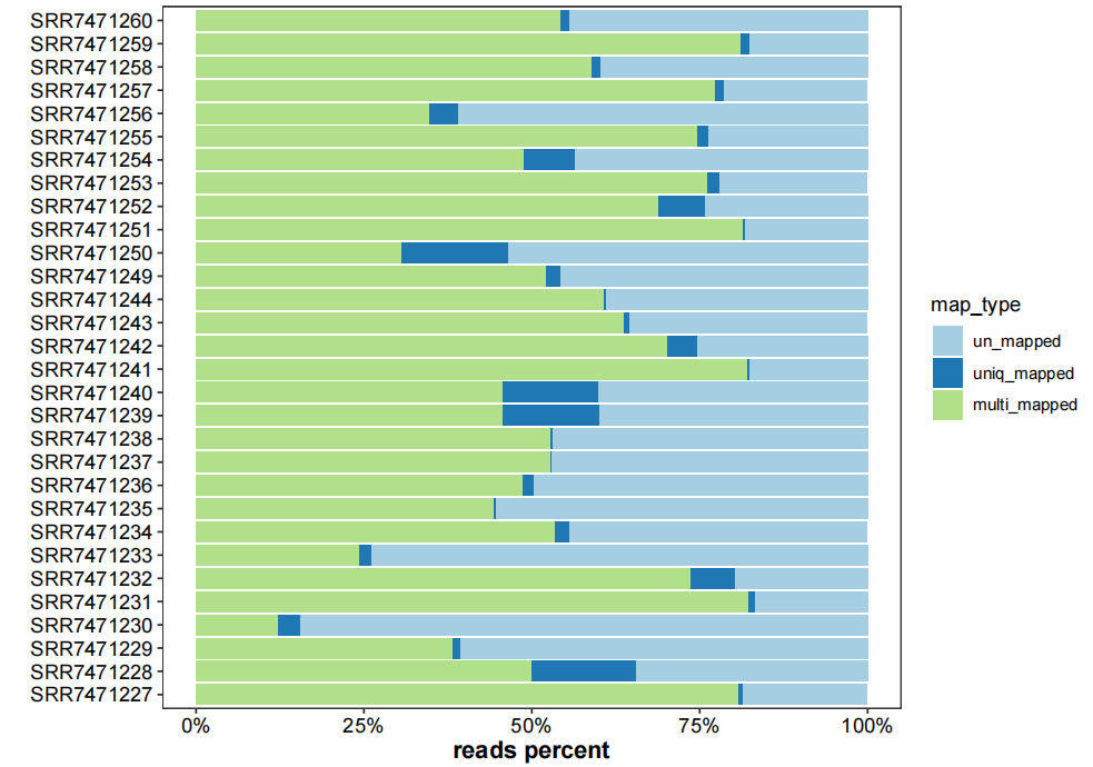
6.6 Map to transcriptome
# ==============================================================================
# map to transcriptome
# ==============================================================================
dir.create("4.map-data")

# batch map to genome
fq_file1 <- list.files("3.rmtrRNA-data/",pattern = ".fq",full.names = T)
output_file <- c('FAS1-trans-rep1','FAS1-inter-rep1','FAS1-trans-rep2','FAS1-inter-rep2',
                 'FAS2-trans-rep1','FAS2-inter-rep1','FAS2-trans-rep2','FAS2-inter-rep2',
                 'FAS1-MPTdel-trans-rep1','FAS1-MPTdel-inter-rep1','FAS1-MPTdel-trans-rep2',
                 'FAS1-MPTdel-trans-rep3','FAS1-MPTdel-inter-rep2','FAS1-MPTdel-inter-rep3',
                 'FAS2-MPTdel-trans-rep1','FAS2-MPTdel-inter-rep1','FAS2-MPTdel-trans-rep2','FAS2-MPTdel-inter-rep2',
                 'GUS1-trans-rep1','GUS1-inter-rep1','GUS1-trans-rep2','GUS1-inter-rep2',
                 'MES1-trans-rep1','MES1-inter-rep1','MES1-trans-rep2','MES1-inter-rep2',
                 'ARC1-trans-rep1','ARC1-inter-rep1','ARC1-trans-rep2','ARC1-inter-rep2')

batch_hisat_align(index = "0.index-data/ref-index/sac_ref",
                  fq_file1 = fq_file1,
                  output_dir = "4.map-data/",
                  output_file = output_file,
                  threads = 24,hisat2_params = list(k = 1))
# ▶ FAS1-trans-rep1 has been processed!
# ▶ FAS1-inter-rep1 has been processed!
# ▶ FAS1-trans-rep2 has been processed!
# ...

# plot mapping info
map_info_geome <- list.files("4.map-data/",pattern = "mapinfo.txt",full.names = TRUE)

plot_mapinfo(mapinfo_file = map_info_geome,
             file_name = sapply(strsplit(map_info_geome,split = "_mapinfo.txt|/"), "[",2))

# plot_mapinfo(mapinfo_file = map_info_geome,
#              file_name = sapply(strsplit(map_info_geome,split = "_mapinfo.txt|/"), "[",2),
#              plot_type = "table")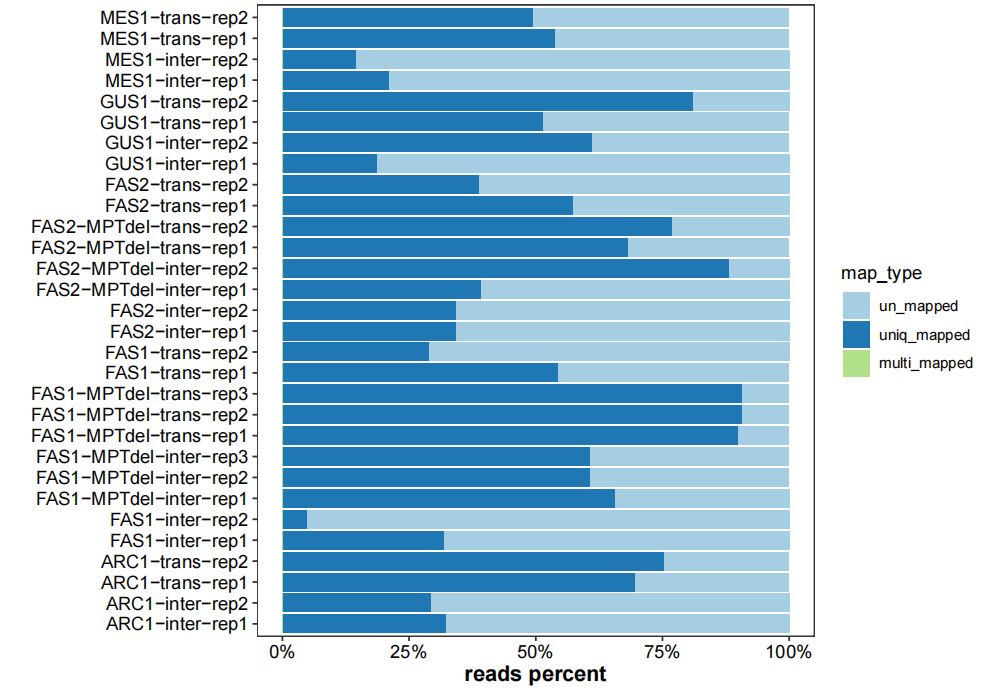
6.7 Ribo QC check
The similar analysis steps like before:
dir.create("5.analysis-data")

setwd("5.analysis-data")
# ==============================================================================
# 1_prepare gene annotation file
# ==============================================================================
# ...
# ==============================================================================
# 2_prepare Ribo QC data
# ==============================================================================
sam_file = list.files("../4.map-data/",pattern = "*sam$",full.names = TRUE)
sample_name <- sapply(strsplit(list.files("../4.map-data/",pattern = "*sam$"),
                               split = ".sam"), "[",1)

# run
pre_qc_data(sam_file = sam_file,
            out_file = paste(sample_name,".qc.txt",sep = ""),
            mapping_type = "transcriptome",
            seq_type = "singleEnd")
# ../4.map-data/ARC1-inter-rep1.sam has been processed!
# ../4.map-data/ARC1-inter-rep2.sam has been processed!
# ../4.map-data/ARC1-trans-rep1.sam has been processed!
# ...

# load qc data
qc_df <- load_qc_data()
qc_df <- qc_df |> dplyr::filter(length >= 20 & length <= 35)

# check
head(qc_df,3)
#   length framest relst framesp relsp feature counts          sample group
# 1     29       1   826       0 -1689       3      1 ARC1-inter-rep1    NA
# 2     24       1   151       0  -306       3      4 ARC1-inter-rep1    NA
# 3     26       1  3118       0  -714       3      1 ARC1-inter-rep1    NA

qc_df$length <- factor(qc_df$length)
qc_df$sample <- factor(qc_df$sample,
                       levels = c('FAS1-trans-rep1','FAS1-trans-rep2',
                                  'FAS2-trans-rep1','FAS2-trans-rep2',
                                  'FAS1-MPTdel-trans-rep1','FAS1-MPTdel-trans-rep2','FAS1-MPTdel-trans-rep3',
                                  'FAS2-MPTdel-trans-rep1','FAS2-MPTdel-trans-rep2',
                                  'GUS1-trans-rep1','GUS1-trans-rep2',
                                  'MES1-trans-rep1','MES1-trans-rep2',
                                  'ARC1-trans-rep1','ARC1-trans-rep2',
                                  'FAS1-inter-rep1','FAS1-inter-rep2',
                                  'FAS2-inter-rep1','FAS2-inter-rep2',
                                  'FAS1-MPTdel-inter-rep1','FAS1-MPTdel-inter-rep2','FAS1-MPTdel-inter-rep3',
                                  'FAS2-MPTdel-inter-rep1','FAS2-MPTdel-inter-rep2',
                                  'GUS1-inter-rep1','GUS1-inter-rep2',
                                  'MES1-inter-rep1','MES1-inter-rep2',
                                  'ARC1-inter-rep1','ARC1-inter-rep2'))
Length distribution:
# length distribution
qc_plot(qc_data = qc_df,type = "length",facet_wrap_list = list(ncol = 5))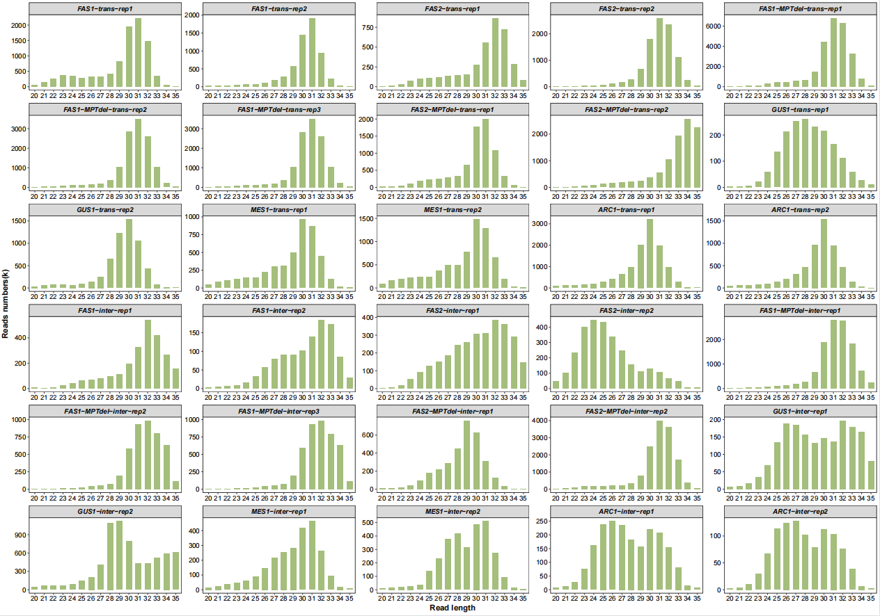
Frames with length distribution:
# length with frame
qc_plot(qc_data = qc_df,type = "length_frame",facet_wrap_list = list(ncol = 5))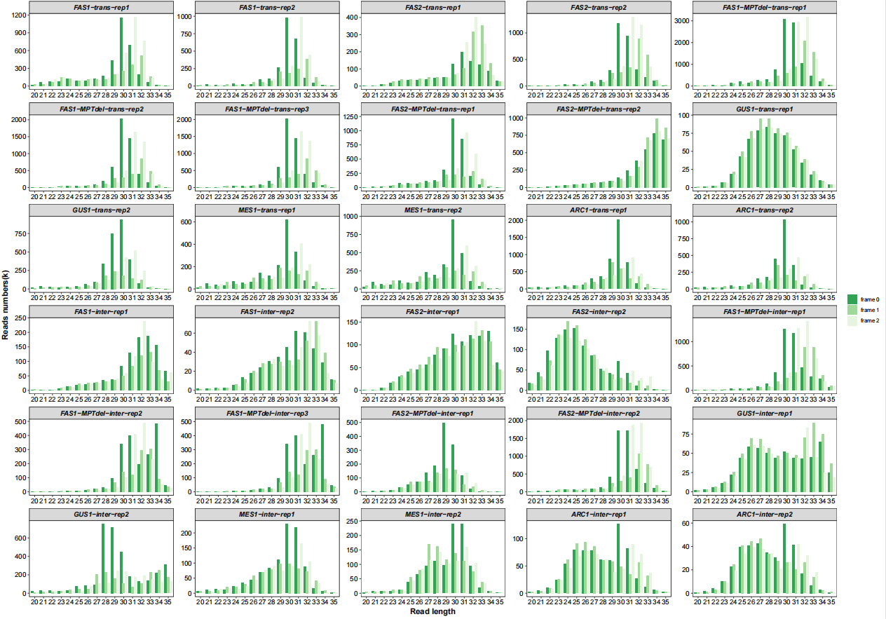
Different region features:
# region features
qc_plot(qc_data = qc_df,type = "feature",facet_wrap_list = list(ncol = 5))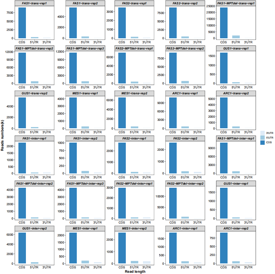
All frames ratio:
# all frames
qc_plot(qc_data = qc_df,type = "frame",facet_wrap_list = list(ncol = 5))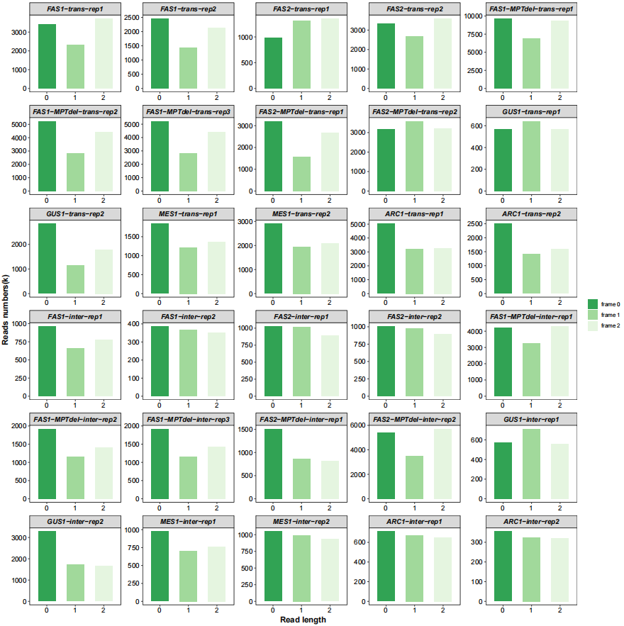
Realtive to start codon with periodicity:
# relative to start/stop site 5x9
rel_to_start_stop(qc_data = qc_df,type = "relst",
                  facet_wrap_list = list(ncol = 5))

# rel_to_start_stop(qc_data = qc_df,type = "relsp",
#                   facet_wrap_list = list(ncol = 5,scales = "fixed"))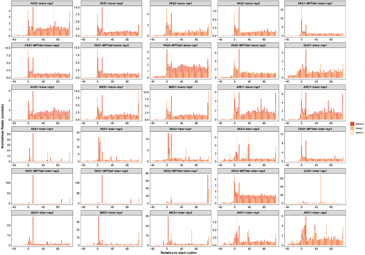
6.8 Calculate ribosome density
# calculate Ribo density
pre_ribo_density_data(sam_file = sam_file,
                      out_file = paste(sample_name,".density.txt",sep = ""),
                      mapping_type = "transcriptome")

# ../4.map-data/ARC1-inter-rep1.sam has been processed!
# ../4.map-data/ARC1-inter-rep2.sam has been processed!
# ../4.map-data/ARC1-trans-rep1.sam has been processed!
# ...
6.9 Enrichment analysis
6.9.1 calculate enrichment ratio
This step calculate the density ratio of factor-bound translatome and total translatome. pre_enrichment_data will calculate enrichment for each transcript positions:
setwd("5.analysis-data")

total <- paste("2.density-data/",
               c('FAS1-trans-rep1','FAS1-trans-rep2',
                 'FAS2-trans-rep1','FAS2-trans-rep2',
                 'FAS1-MPTdel-trans-rep1','FAS1-MPTdel-trans-rep2','FAS1-MPTdel-trans-rep3',
                 'FAS2-MPTdel-trans-rep1','FAS2-MPTdel-trans-rep2',
                 'GUS1-trans-rep1','GUS1-trans-rep2',
                 'MES1-trans-rep1','MES1-trans-rep2',
                 'ARC1-trans-rep1','ARC1-trans-rep2'),
               ".density.txt",sep = "")

ip <- paste("2.density-data/",
            c('FAS1-inter-rep1','FAS1-inter-rep2',
              'FAS2-inter-rep1','FAS2-inter-rep2',
              'FAS1-MPTdel-inter-rep1','FAS1-MPTdel-inter-rep2','FAS1-MPTdel-inter-rep3',
              'FAS2-MPTdel-inter-rep1','FAS2-MPTdel-inter-rep2',
              'GUS1-inter-rep1','GUS1-inter-rep2',
              'MES1-inter-rep1','MES1-inter-rep2',
              'ARC1-inter-rep1','ARC1-inter-rep2'),
            ".density.txt",sep = "")

# calculate enrich ratio
dir.create("3.enrich-data")

# output
out_file <- paste("3.enrich-data/",
                  c("FAS1-rep1","FAS1-rep2","FAS2-rep1","FAS2-rep2",
                    "FAS1-MPTdel-rep1","FAS1-MPTdel-rep2","FAS1-MPTdel-rep3",
                    "FAS2-MPTdel-rep1","FAS2-MPTdel-rep2",
                    "GUS1-rep1","GUS1-rep2","MES1-rep1","MES1-rep2","ARC1-rep1","ARC1-rep2"),
                  ".enrich.txt",sep = "")

# run
pre_enrichment_data(riboIP_file = ip,
                    riboInput_file = total,
                    output_file = out_file)
# 3.enrich-data/FAS1-rep1.enrich.txt has been processed!
# 3.enrich-data/FAS1-rep2.enrich.txt has been processed!
# 3.enrich-data/FAS2-rep1.enrich.txt has been processed!
# ...
6.9.2 track plot
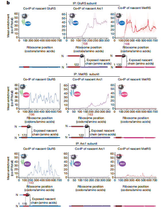
First we show the raw seRP figure from paper:
You can still use track_plot to visualize the output:
# ==============================================================================
# load data and visualize
# ==============================================================================
df_fasx <- load_enrich_data(enrich_data = c("3.enrich-data/ARC1-rep1.enrich.txt",
                                            "3.enrich-data/ARC1-rep2.enrich.txt",
                                            "3.enrich-data/GUS1-rep1.enrich.txt",
                                            "3.enrich-data/GUS1-rep2.enrich.txt",
                                            "3.enrich-data/MES1-rep1.enrich.txt",
                                            "3.enrich-data/MES1-rep2.enrich.txt"),
                            gene_names = c('ARC1','GUS1','MES1'),
                            sample_name = c("ARC1","ARC1","GUS1","GUS1","MES1","MES1"))

# check
head(df_fasx,3)
# # A tibble: 3 × 7
# # Groups:   gene_name, trans_id, codon_pos, type [1]
#   gene_name trans_id     codon_pos type  sample density density_sd
#   <chr>     <chr>            <int> <chr> <chr>    <dbl>      <dbl>
# 1 ARC1      YGL105W_mRNA         1 ribo  ARC1     0.690     0.976
# 2 ARC1      YGL105W_mRNA         1 ribo  GUS1     0.796     0.0103
# 3 ARC1      YGL105W_mRNA         1 ribo  MES1     0.868     0.888

# plot 6x10
track_plot(plot_type = "interactome",
           signal_data = df_fasx,
           gene_order = c('GUS1','ARC1','MES1'),
           sample_order = c('GUS1','MES1','ARC1'),
           line_col = c('GUS1' = '#4883C6','ARC1' = '#AA356A','MES1' = '#D52C30'),
           remove_trans_panel_border = T)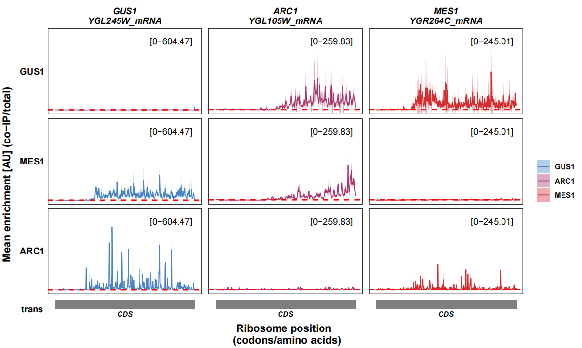
6.9.3 enrichment with slide window
In the article, author used a slide window with 20nt to smooth the enrichment density:
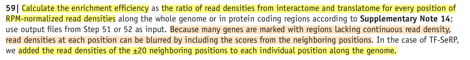
You can also do this with pre_slideWindow_enrichment_data function.
# calculate enrich ratio
dir.create("4.swEnrich-data")

total <- paste("2.density-data/",
               c('GUS1-trans-rep1','GUS1-trans-rep2',
                 'MES1-trans-rep1','MES1-trans-rep2',
                 'ARC1-trans-rep1','ARC1-trans-rep2'),
               ".density.txt",sep = "")

ip <- paste("2.density-data/",
            c('GUS1-inter-rep1','GUS1-inter-rep2',
              'MES1-inter-rep1','MES1-inter-rep2',
              'ARC1-inter-rep1','ARC1-inter-rep2'),
            ".density.txt",sep = "")

# output
out_file <- paste("4.swEnrich-data/",
                  c("GUS1-rep1","GUS1-rep2","MES1-rep1","MES1-rep2","ARC1-rep1","ARC1-rep2"),
                  ".enrich.txt",sep = "")

# run
pre_slideWindow_enrichment_data(riboIP_file = ip,
                                riboInput_file = total,
                                gene_list = c('GUS1','ARC1','MES1'),
                                output_file = out_file)
Visualize data:
# ==============================================================================
# load data and visualize
# ==============================================================================
file <- list.files("4.swEnrich-data/","*.txt",full.names = T)
file
# [1] "4.swEnrich-data/ARC1-rep1.enrich.txt" "4.swEnrich-data/ARC1-rep2.enrich.txt"
# [3] "4.swEnrich-data/GUS1-rep1.enrich.txt" "4.swEnrich-data/GUS1-rep2.enrich.txt"
# [5] "4.swEnrich-data/MES1-rep1.enrich.txt" "4.swEnrich-data/MES1-rep2.enrich.txt"

df_sw <- load_enrich_data(data_type = "sw",
                            enrich_data = file,
                            sample_name = c("ARC1","ARC1","GUS1","GUS1","MES1","MES1"))

# check
head(df_sw[1:3,])
# # A tibble: 3 × 7
# # Groups:   gene_name, trans_id, codon_pos, type [1]
# gene_name trans_id     codon_pos type  sample density density_sd
# <chr>     <chr>            <dbl> <chr> <chr>    <dbl>      <dbl>
# 1 ARC1      YGL105W_mRNA         1 ribo  ARC1      1.82     0.152
# 2 ARC1      YGL105W_mRNA         1 ribo  GUS1      1.49     0.0293
# 3 ARC1      YGL105W_mRNA         1 ribo  MES1      2.09     1.33

# plot 6x10
track_plot(plot_type = "interactome",
           signal_data = df_sw,
           gene_order = c('GUS1','ARC1','MES1'),
           sample_order = c('GUS1','MES1','ARC1'),
           line_col = c('GUS1' = '#4883C6','ARC1' = '#AA356A','MES1' = '#D52C30'),
           remove_trans_panel_border = T)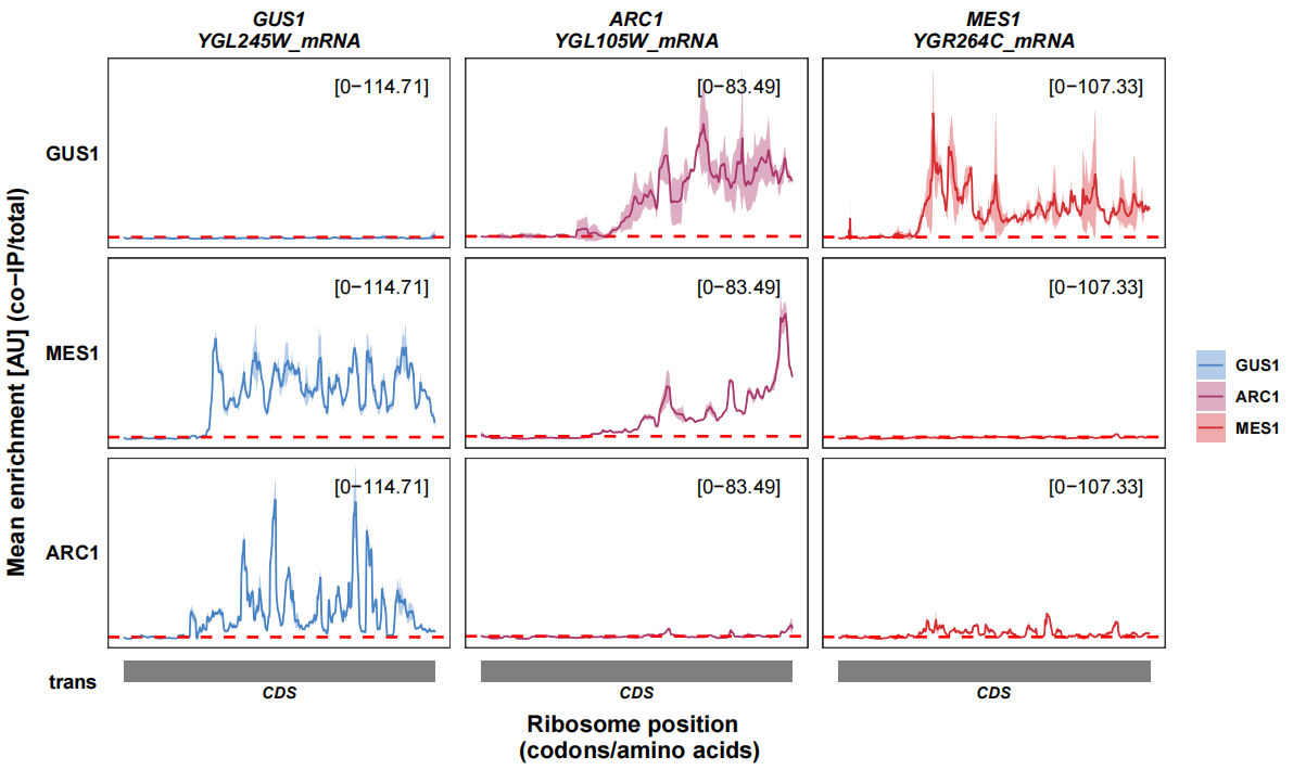
This looks much better!