Chapter 3 dotplotGsea
dotplotGsea can be used to show GSEA results with a scatter plot.
Get a enriched object:
library(clusterProfiler)
library(org.Hs.eg.db)

# loda genelist
data(geneList, package="DOSE")

# enrichment
ego3 <- gseGO(geneList     = geneList,
              OrgDb        = org.Hs.eg.db,
              ont          = "BP",
              minGSSize    = 100,
              maxGSSize    = 500,
              pvalueCutoff = 0.05,
              verbose      = FALSE)
Show the top 10 terms:
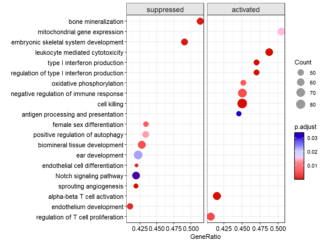
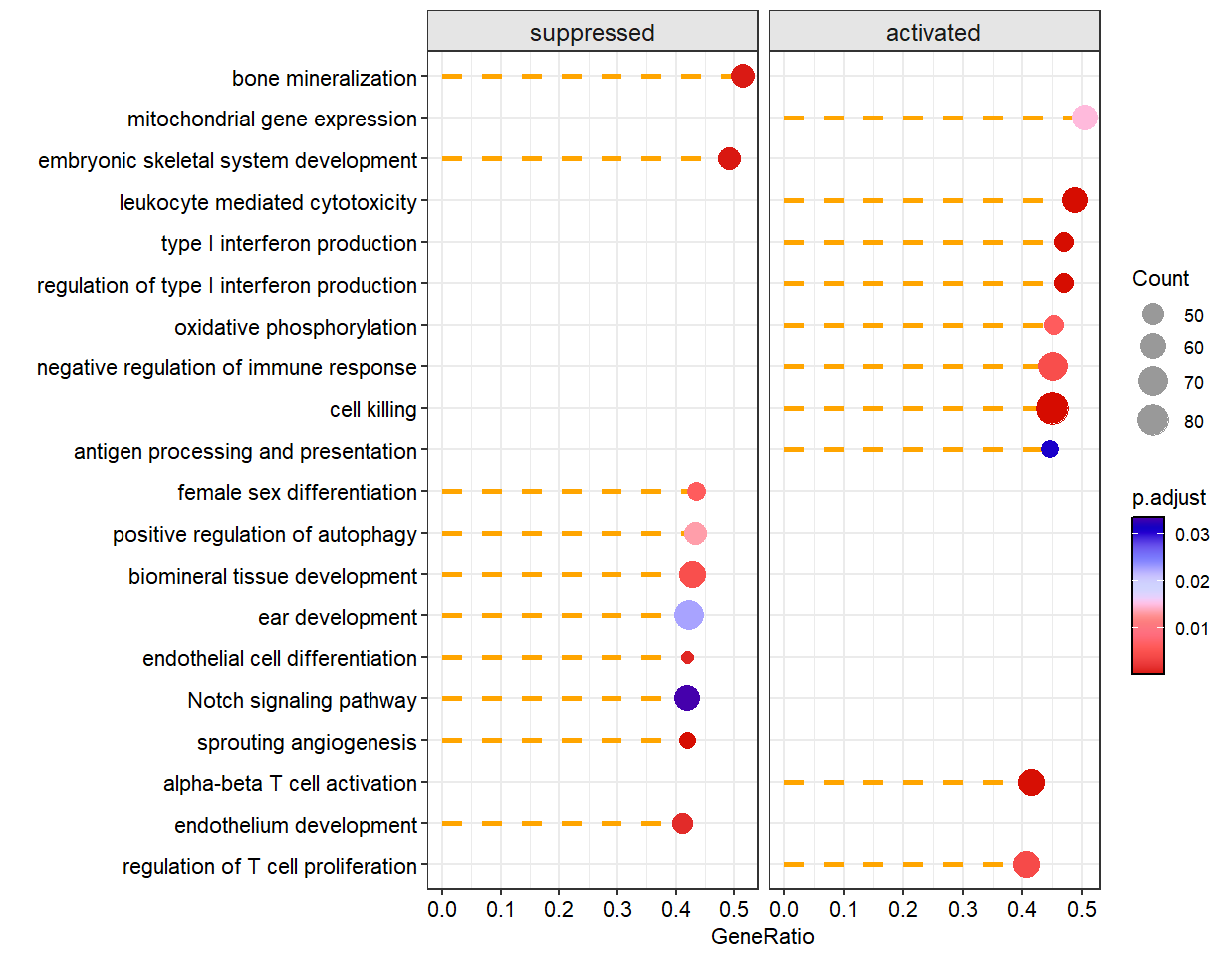
# default plot
dotplotGsea(data = ego3,topn = 10)
# $df
# # A tibble: 20 × 14
# # Groups:   type [2]
# ID         Description   setSize enrichmentScore   NES  pvalue p.adjust  qvalue  rank leading_edge
# <chr>      <fct>           <int>           <dbl> <dbl>   <dbl>    <dbl>   <dbl> <dbl> <chr>
#   1 GO:0042129 regulation o…     150           0.358  1.54 8.43e-4  4.21e-3 2.22e-3  2741 tags=41%, l…
# 2 GO:0003158 endothelium …     117          -0.452 -1.73 2.12e-4  1.37e-3 7.25e-4  2839 tags=41%, l…
# 3 GO:0046631 alpha-beta T…     147           0.426  1.83 1.09e-5  1.09e-4 5.74e-5  2570 tags=41%, l…
# 4 GO:0002040 sprouting an…     105          -0.499 -1.89 6.61e-6  6.91e-5 3.65e-5  2696 tags=42%, l…
# 5 GO:0007219 Notch signal…     143          -0.352 -1.40 1.24e-2  3.34e-2 1.77e-2  3914 tags=42%, l…
# 6 GO:0045446 endothelial …     100          -0.479 -1.80 1.65e-4  1.10e-3 5.78e-4  2839 tags=42%, l…
# 7 GO:0043583 ear developm…     168          -0.354 -1.43 7.54e-3  2.29e-2 1.21e-2  3373 tags=42%, l…
# 8 GO:0031214 biomineral t…     145          -0.395 -1.57 1.00e-3  4.80e-3 2.53e-3  2101 tags=43%, l…
# 9 GO:0010508 positive reg…     120          -0.404 -1.56 3.94e-3  1.34e-2 7.08e-3  3747 tags=43%, l…
# 10 GO:0046660 female sex d…     106          -0.427 -1.62 1.43e-3  6.36e-3 3.36e-3  3148 tags=43%, l…
# 11 GO:0019882 antigen proc…     101           0.356  1.43 1.12e-2  3.09e-2 1.63e-2  3147 tags=45%, l…
# 12 GO:0001906 cell killing      180           0.464  2.05 1.31e-8  3.08e-7 1.63e-7  2616 tags=45%, l…
# 13 GO:0050777 negative reg…     162           0.349  1.53 9.28e-4  4.59e-3 2.42e-3  3282 tags=45%, l…
# 14 GO:0006119 oxidative ph…     104           0.394  1.59 1.42e-3  6.34e-3 3.35e-3  3703 tags=45%, l…
# 15 GO:0032479 regulation o…     100           0.493  1.97 1.54e-6  1.94e-5 1.02e-5  2932 tags=47%, l…
# 16 GO:0032606 type I inter…     100           0.493  1.97 1.54e-6  1.94e-5 1.02e-5  2932 tags=47%, l…
# 17 GO:0001909 leukocyte me…     121           0.475  1.97 1.34e-6  1.75e-5 9.23e-6  2746 tags=49%, l…
# 18 GO:0048706 embryonic sk…     106          -0.483 -1.83 5.13e-5  4.04e-4 2.13e-4  2919 tags=49%, l…
# 19 GO:0140053 mitochondria…     115           0.361  1.49 4.44e-3  1.49e-2 7.85e-3  4006 tags=50%, l…
# 20 GO:0030282 bone mineral…     105          -0.469 -1.78 6.46e-5  4.84e-4 2.56e-4  3348 tags=51%, l…
# # ℹ 4 more variables: core_enrichment <chr>, type <fct>, Count <int>, GeneRatio <dbl>
#
# $plot
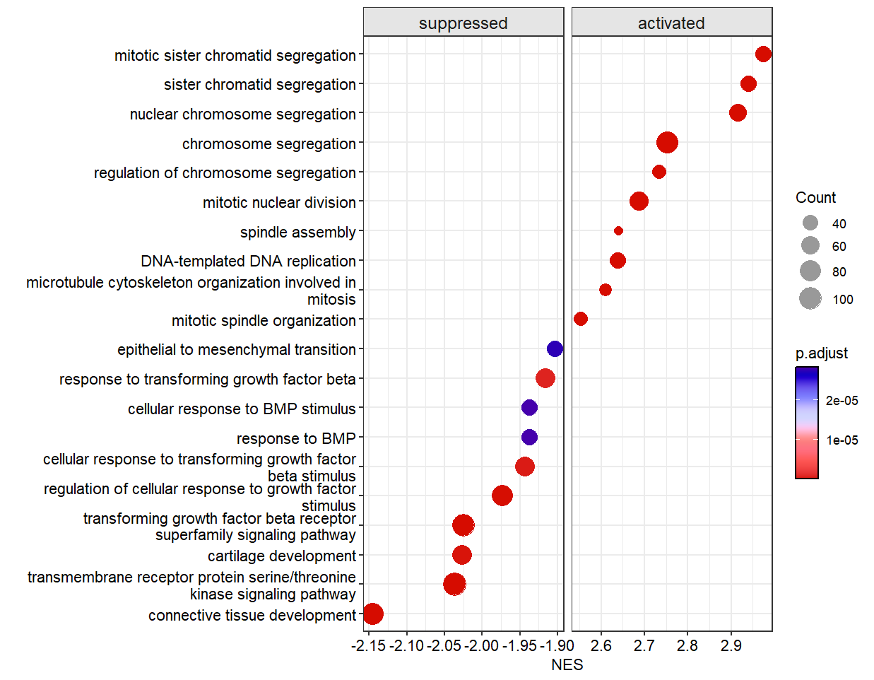
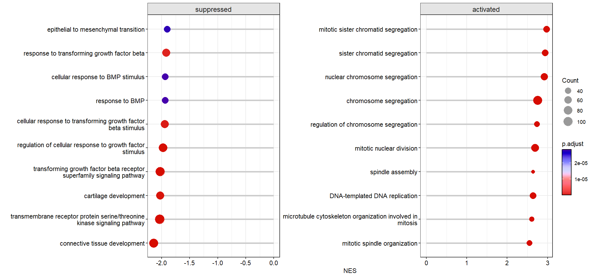
Use NES as the X axis:
Make lollipop plot:
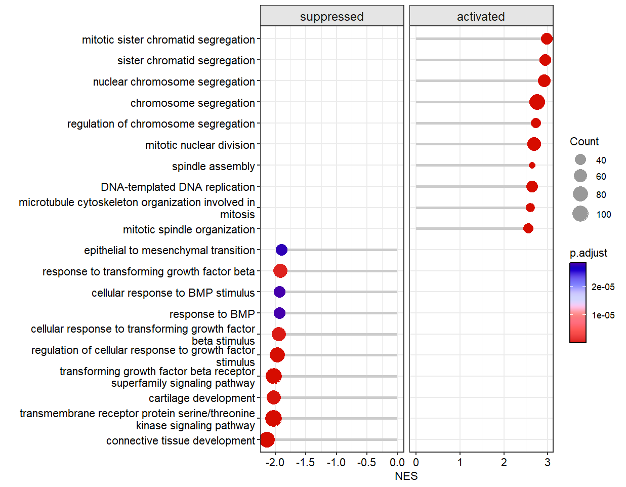
Add dash line:
# change line style
dotplotGsea(data = ego3,topn = 10,
            add.seg = T,
            line.col = 'orange',
            line.type = 'dashed')
Free scale for each sub plot:
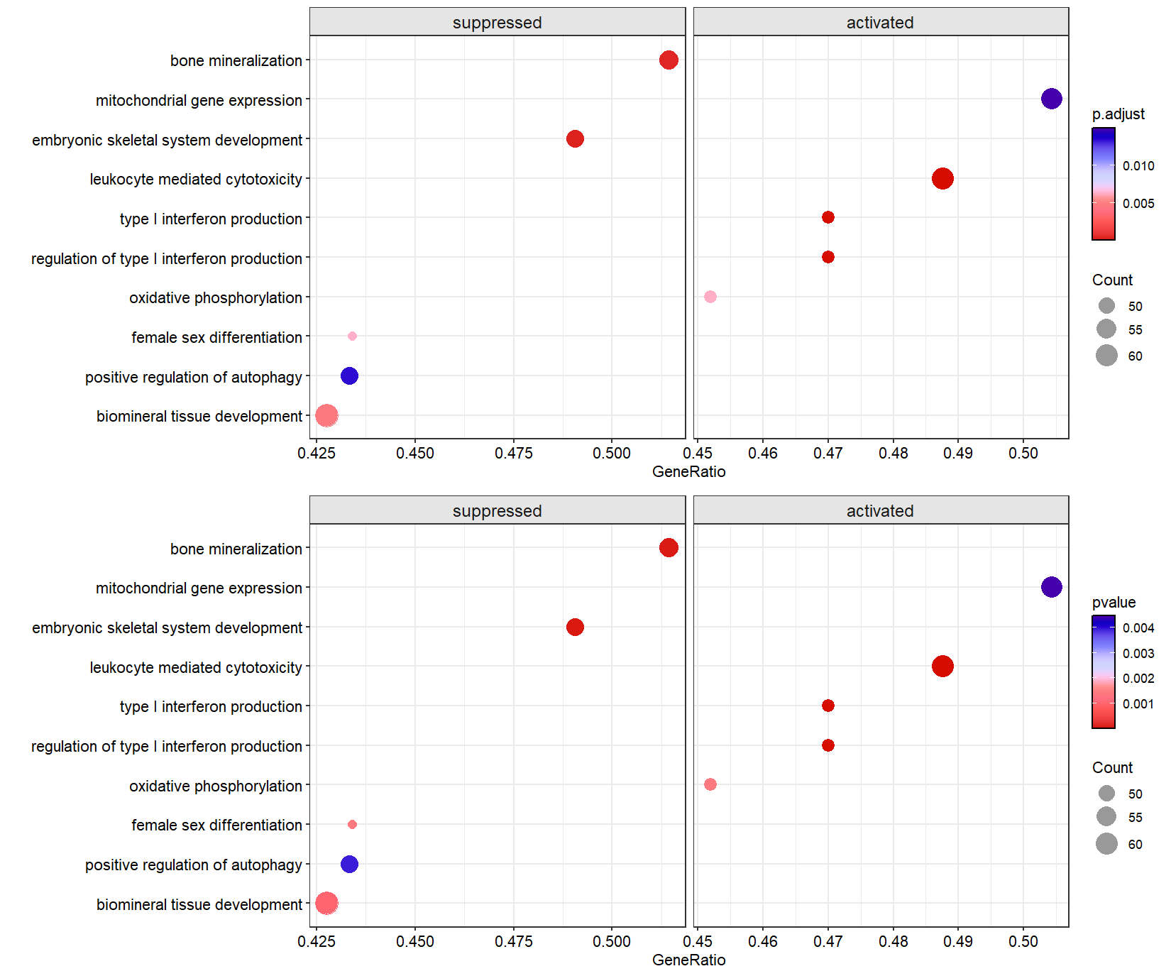
Control the pvalue and p.adjusted value cutoff:
p1 <- dotplotGsea(data = ego3,topn = 5,
                  pajust = 0.1)$plot

p2 <- dotplotGsea(data = ego3,topn = 5,
                  pval = 0.05)$plot

# combine
cowplot::plot_grid(p1,p2,nrow = 2,align = 'hv')