Chapter 6 Parse output results from GSEA software
GseaVis can also parse GSEA software output resluts and re-draw the data to supply a publication-quality plot.
6.2 Parse GSEA results
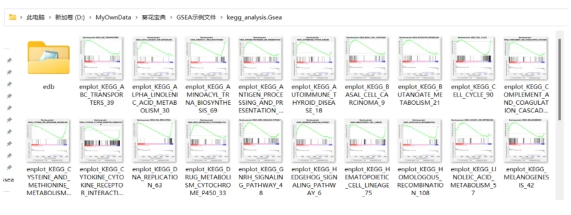
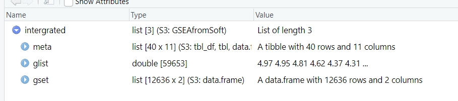
readGseaFile can parse the GSEA software output directory and return a list containing multiple results about enrichment:
intergrated <- readGseaFile(filePath = "kegg_analysis.Gsea/")
str(intergrated)
# $meta
# # A tibble: 40 × 11
# ID            Description setSize enrichmentScore   NES  pvalue p.adjust qvalue  rank leading_edge
# <chr>         <chr>         <dbl>           <dbl> <dbl>   <dbl>    <dbl>  <dbl> <dbl> <chr>
#   1 KEGG_DNA_REP… KEGG_DNA_R…      36          -0.742 -1.65 0.00196    0.108  0.1    5640 tags=72%, l…
# 2 KEGG_PYRIMID… KEGG_PYRIM…      97          -0.612 -1.58 0.00178    0.176  0.291  8892 tags=52%, l…
# 3 KEGG_AMINOAC… KEGG_AMINO…      41          -0.686 -1.55 0.00914    0.179  0.412  8244 tags=56%, l…
# 4 KEGG_CYSTEIN… KEGG_CYSTE…      34          -0.683 -1.49 0.0148     0.298  0.682  9190 tags=59%, l…
# 5 KEGG_HEMATOP… KEGG_HEMAT…      85          -0.596 -1.49 0.00515    0.257  0.715  4563 tags=26%, l…
# 6 KEGG_RNA_POL… KEGG_RNA_P…      28          -0.714 -1.49 0.0120     0.215  0.717  8772 tags=64%, l…
# 7 KEGG_RNA_DEG… KEGG_RNA_D…      59          -0.624 -1.48 0.00530    0.204  0.752 14222 tags=64%, l…
# 8 KEGG_PROTEAS… KEGG_PROTE…      46          -0.637 -1.48 0.0125     0.181  0.758 13047 tags=65%, l…
# 9 KEGG_PROXIMA… KEGG_PROXI…      23          -0.734 -1.47 0.0343     0.175  0.775  7113 tags=52%, l…
# 10 KEGG_CELL_CY… KEGG_CELL_…     124          -0.541 -1.45 0.00350    0.203  0.862  8600 tags=44%, l…
# # ℹ 30 more rows
# # ℹ 1 more variable: core_enrichment <chr>
# # ℹ Use `print(n = ...)` to see more rows
#
# $glist
# AC068790.9     AC135048.2     AC142381.2           DGKI        TMEM265       RPL18P10
# 4.968889       4.951065       4.811294       4.624895       4.367372       4.308214
# MKRN9P           NPNT        C1orf21         TSPAN7       GOLGA8IP        ADAMTS9
Check the resuts:
# check enrichment data
head(intergrated$meta[1:3,1:5])
# # A tibble: 3 × 5
#   ID                               Description                      setSize enrichmentScore   NES
#   <chr>                            <chr>                              <dbl>           <dbl> <dbl>
# 1 KEGG_DNA_REPLICATION             KEGG_DNA_REPLICATION                  36          -0.742 -1.65
# 2 KEGG_PYRIMIDINE_METABOLISM       KEGG_PYRIMIDINE_METABOLISM            97          -0.612 -1.58
# 3 KEGG_AMINOACYL_TRNA_BIOSYNTHESIS KEGG_AMINOACYL_TRNA_BIOSYNTHESIS      41          -0.686 -1.55

# check gene lists
head(intergrated$glist)
# AC068790.9 AC135048.2 AC142381.2       DGKI    TMEM265   RPL18P10
#   4.968889   4.951065   4.811294   4.624895   4.367372   4.308214

# check terms
head(intergrated$gset[1:3,])
#                   term  gene
# 1 KEGG_DNA_REPLICATION  DNA2
# 2 KEGG_DNA_REPLICATION POLE4
# 3 KEGG_DNA_REPLICATION POLE3
Or you can also supply the path to gseaNb directlly:
setid <- c("KEGG_RIBOSOME",
"KEGG_HEDGEHOG_SIGNALING_PATHWAY",
"KEGG_DNA_REPLICATION",
"KEGG_PYRIMIDINE_METABOLISM")
# plot
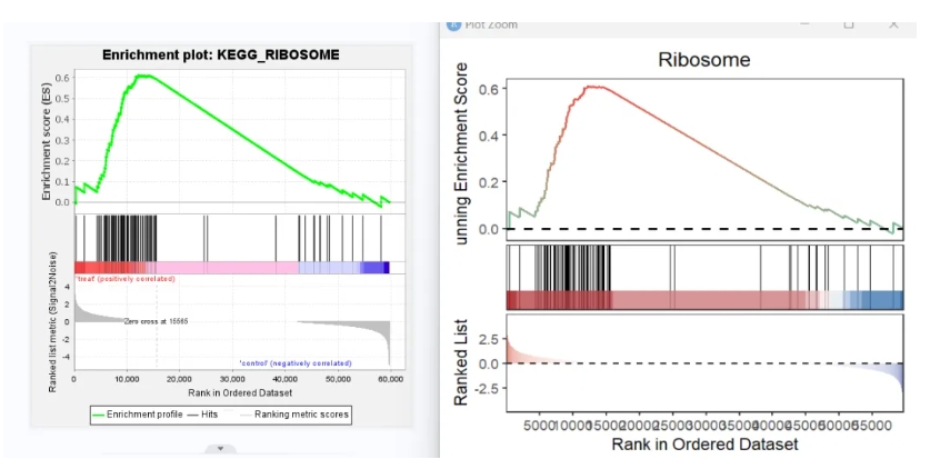
gseaNb(filePath = "kegg_analysis.Gsea/",
geneSetID = setid[1])
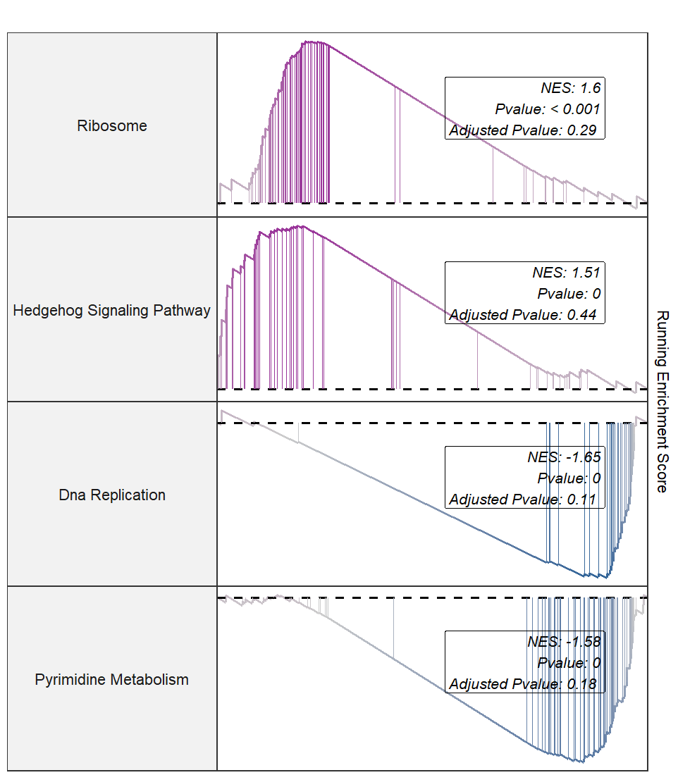
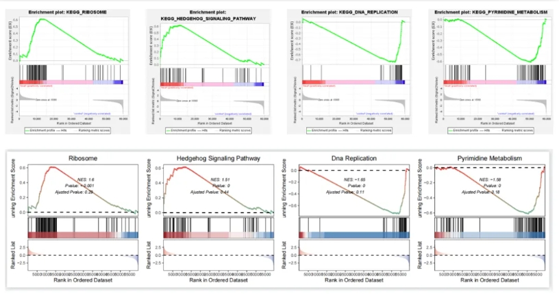
Lets compare the other terms:
lapply(1:4, function(x){
  gseaNb(filePath = intergrated,
         geneSetID = setid[x],
         addPval = T,
         pvalX = 0.6,
         pvalY = 0.6)
}) -> plist
# combine
cowplot::plot_grid(plotlist = plist,nrow = 1,align = 'hv')
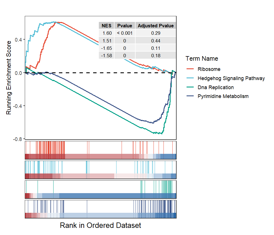
Multiple terms plot:
# multiple terms
gseaNb(filePath = intergrated,
       geneSetID = setid,
       curveCol = ggsci::pal_npg()(4),
       subPlot = 2,
       addPval = T,
       pvalX = 1,
       pvalY = 1)
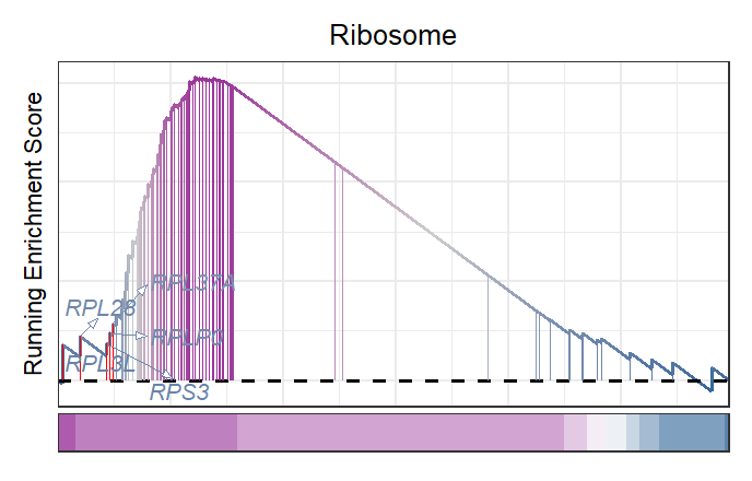
New style plot:
# new style plot
gseaNb(filePath = intergrated,
       geneSetID = setid[1],
       newGsea = T,
       addGene = T,
       markTopgene = T)
Multiple facet plot:
# multiple terms of new style
gseaNb(filePath = intergrated,
       geneSetID = setid,
       newGsea = T,
       rmHt = T,
       addPval = T,
       pvalX = 0.9,
       pvalY = 0.6)