metagene_plot(object = obj0)15 Metagene plot
15.1 Average ribosome occupancy around start or stop codons
15.1.1 Visualizing global initiation and termination trends
In Ribo-seq analysis, the metagene plot is a widely used tool to visualize the average ribosome occupancy near translation start or stop codons across transcripts. By aggregating reads from a large set of coding sequences (CDSs), it reveals global patterns in translation initiation or termination.
Ribosomes are expected to accumulate at the start codon during initiation, and in certain conditions, near the stop codon during termination or ribosome stalling. Examining these patterns provides insight into translational dynamics, data quality, and the fidelity of P-site assignment.
15.1.2 What does metagene_plot() show?
The metagene_plot() function generates a smoothed line plot showing average ribosome occupancy (normalized read density) relative to either:
The start codon (type = “rel2start”), or
The stop codon (type = “rel2stop”)
Visualization is performed in either nucleotide (nt) or codon scale, across all coding sequences that pass user-defined filters for length and minimum counts.
What the plot displays:
X-axis: Distance from start/stop codon (in nt or codon units)
Y-axis: Average normalized ribosome occupancy
Facets: One line per sample or sample group (with replicates optionally merged)
This metagene-level alignment enables detection of global features such as:
Ribosomal accumulation at initiation sites (initiation peaks)
Periodicity along coding regions (indicative of translation elongation)
Ribosome drop-off or stalling near stop codons
15.1.3 Normalization approaches
Normalization helps adjust for transcript length, library size, and gene-level expression. Two approaches are supported:
average: raw read counts normalized by CDS length and transcript-specific mean coverage
tpm: TPM-like normalization using reads per kilobase (RPK) divided by sample-level totals
These methods ensure that highly expressed CDSs do not dominate the signal, allowing for unbiased meta-level averages.
15.1.4 Additional controls & filters
do_offset_correct: Apply a position shift to correct P-site offset (optional)
read_length: Select only ribosome footprint fragment sizes of interest
exclude_length: Exclude regions near CDS boundaries to avoid ambiguous mapping
min_cds_length: Filter out short CDSs (e.g. <600 nt)
min_counts: Require minimum read support per transcript
facet_wrap: Customize the faceting layout (e.g. by sample or condition)
merge_rep: Aggregate replicates of the same sample group for cleaner profiles
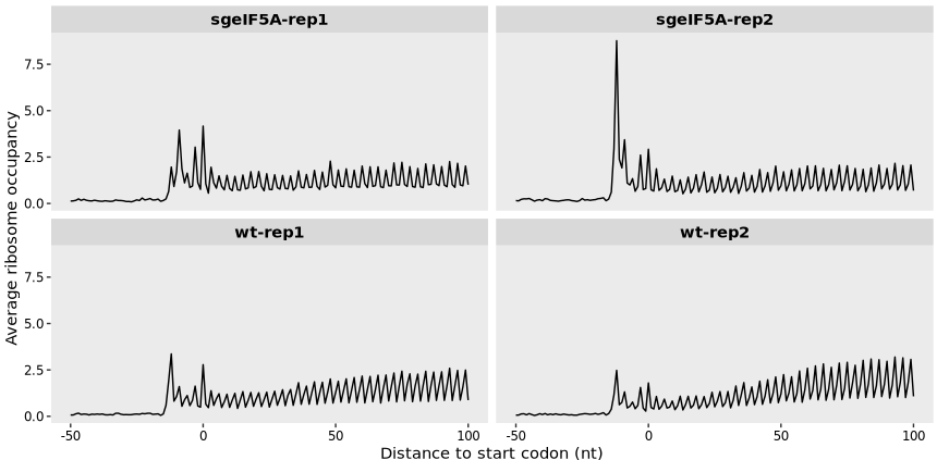
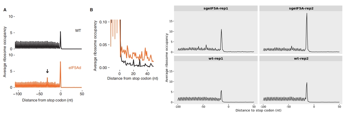
15.1.5 Example : metagene plot centered at start codon
A noticeable increase in ribosome occupancy around the start codon is observed upon eIF5A knockout compared to the wild-type (WT), suggesting enhanced ribosome accumulation at translation initiation sites:
By setting mode = “codon”, the unit of relative position is converted from nucleotides (nt) to codons. The rel2st_dist parameter defines the positional window around the start codon. As shown, the overall trend remains consistent with the original nucleotide-based plot:
metagene_plot(object = obj0,
              mode = "codon",
              rel2st_dist = c(-50, 900))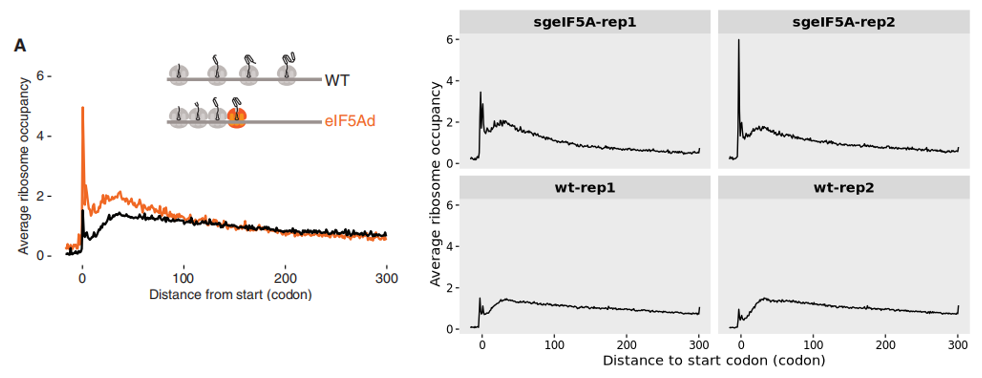
The ribosome occupancy profile, aligned relative to the stop codon, displays the averaged translation read density across transcripts within the defined region. Notably, in the eIF5A knockout condition, a marked increase in ribosome occupancy is observed near the stop codon, suggesting enhanced ribosome stalling or delayed termination compared to the wild-type:
metagene_plot(object = obj0,
              type = "rel2stop",
              mode = "codon",
              rel2sp_dist = c(-900, 50))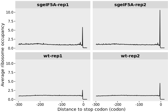
The authors also observed that loss of eIF5A impairs translation termination, as indicated by a clear ribosome stalling peak approximately 30 nucleotides(offset corrected) upstream of the stop codon:
15.2 Method to aggregate data for each position
The metagene_plot function supports three aggregation methods (“median”, “mean” and “sum”) to summarize ribosome‐density signals at each transcript position. Users can choose the method that best fits their analysis goals. The example data shown here are taken from the “Profiling-Ssb-Nascent-Chain” section—see that vignette for the complete data‐processing workflow:
library(ggplot2)

metagene_plot(object = obj,
              mode = "codon",
              rel2st_dist = c(-50, 1500),
              facet_wrap = ggplot2::facet_wrap(~sample,nrow = 2),
              method = "median")
Set method = “mean”:
metagene_plot(object = obj,
              mode = "codon",
              rel2st_dist = c(-50, 1500),
              facet_wrap = ggplot2::facet_wrap(~sample,nrow = 2),
              method = "mean")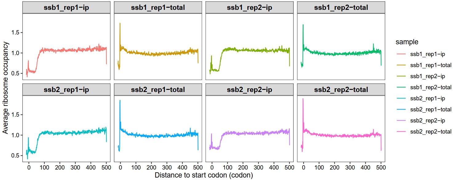
Set method = “sum”:
metagene_plot(object = obj,
              mode = "codon",
              rel2st_dist = c(-50, 1500),
              facet_wrap = ggplot2::facet_wrap(~sample,nrow = 2),
              method = "sum")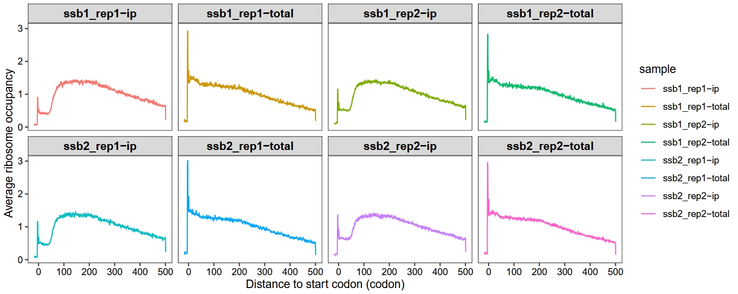
Merge replicates:
metagene_plot(object = obj,
              mode = "codon",
              rel2st_dist = c(-50, 1500),
              method = "median",
              merge_rep = T)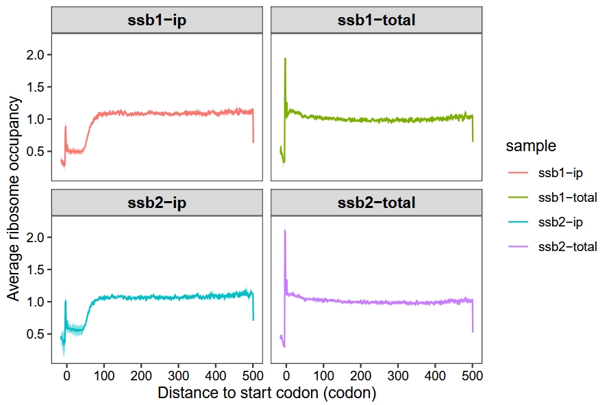
Do 1000 bootstraps to add 95% confidence intervals:
metagene_plot(object = obj,
              mode = "codon",
              rel2st_dist = c(-50, 1500),
              method = "median",
              facet_wrap = ggplot2::facet_wrap(~sample,nrow = 2),
              do_bootstrap = T)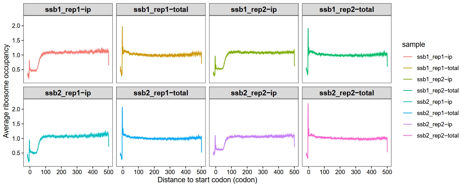
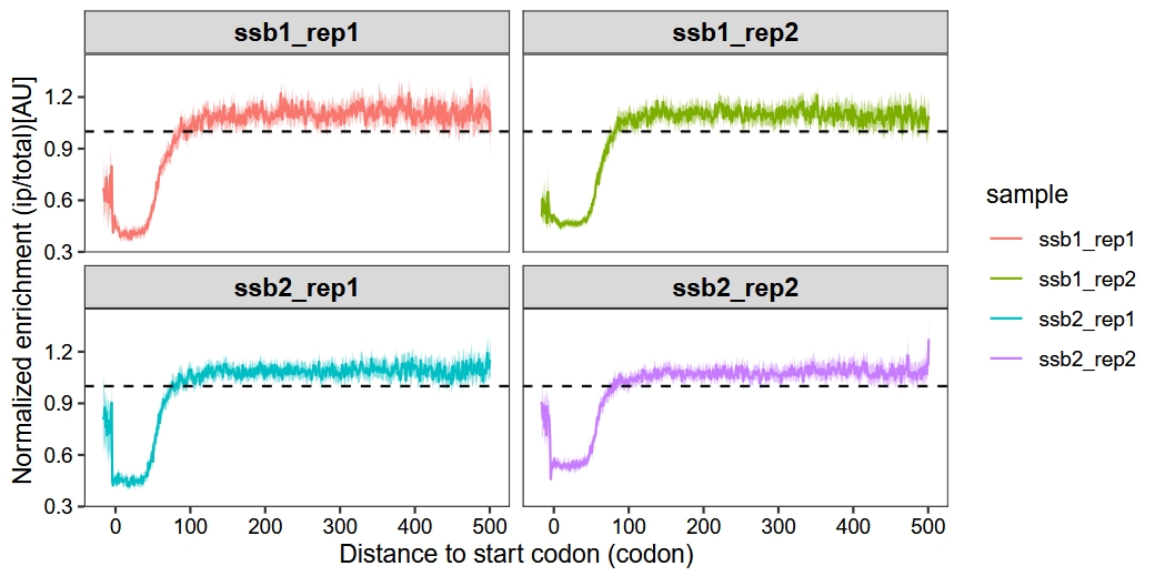
15.3 Enrichment metagene analysis
We create metagene plots by analyzing the ratio of ribosome density in IP samples compared to total samples at positions relative to start codons or stop codons across genes from selective ribosome profiling data. The enrichment_metagene_plot function maintains most parameters consistent with the metagene_plot function.
Default plot:
enrichment_metagene_plot(object = obj,
                         mode = "codon",
                         rel2st_dist = c(-50, 1500),
                         facet_wrap = ggplot2::facet_wrap(~sample,nrow = 2),
                         method = "median")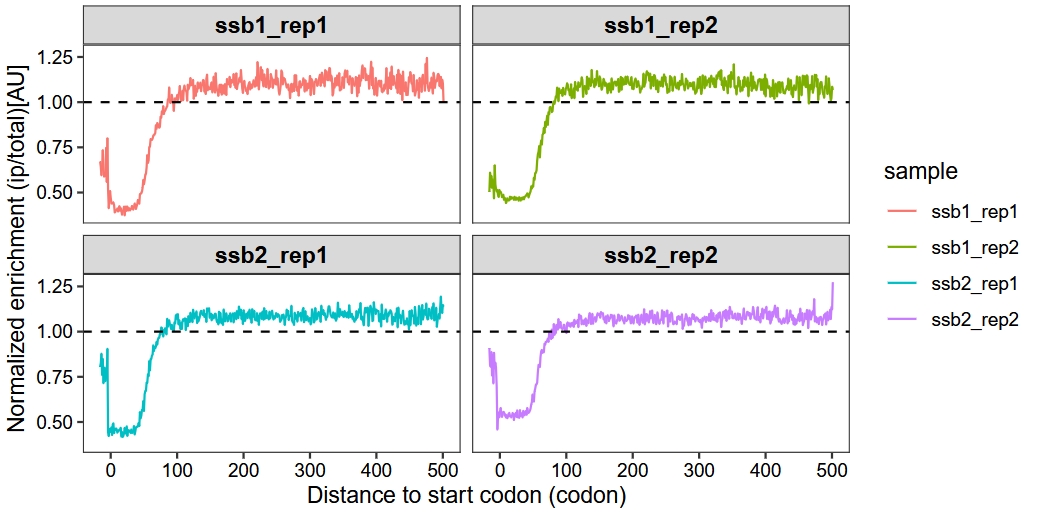
Set method = “sum”:
enrichment_metagene_plot(object = obj,
                         mode = "codon",
                         rel2st_dist = c(-50, 1500),
                         facet_wrap = ggplot2::facet_wrap(~sample,nrow = 2),
                         method = "sum")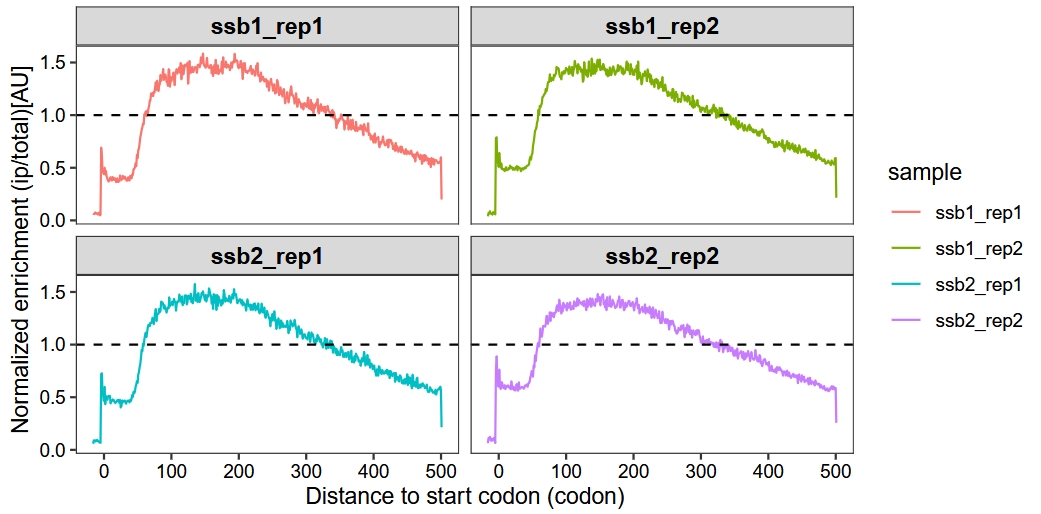
Merge replicates:
enrichment_metagene_plot(object = obj,
                         mode = "codon",
                         rel2st_dist = c(-50, 1500),
                         method = "median",
                         merge_rep = T)
Do bootstraps to add 95% confidence interval:
enrichment_metagene_plot(object = obj,
                         mode = "codon",
                         rel2st_dist = c(-50, 1500),
                         method = "median",
                         facet_wrap = ggplot2::facet_wrap(~sample,nrow = 2),
                         do_bootstrap = T)