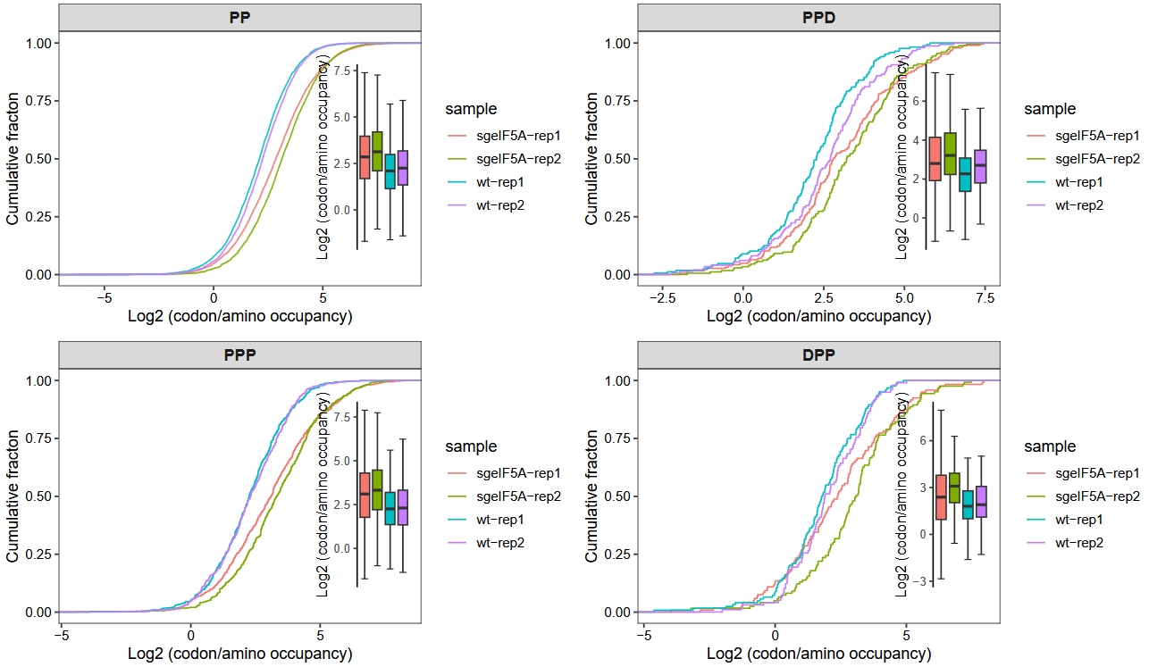
motif_occupancy(object = obj0,
                cds_fa = "./sac_cds.fa",
                search_type = "amino",
                do_offset_correct = T,
                motif_pattern = c("PP","PPP","PPD","DPP"))
# `summarise()` has grouped output by 'sample', 'rname'. You can override using the `.groups` argument.
# $plot
#
# $statistics
# # A tibble: 24 × 9
# codon_seq .y.   group1       group2               p     p.adj p.format p.signif method
# <chr>     <chr> <chr>        <chr>            <dbl>     <dbl> <chr>    <chr>    <chr>
# 1 PP        value sgeIF5A-rep1 sgeIF5A-rep2 5.52e- 17 8.80e- 16 < 2e-16  ****     Wilcoxon
# 2 PP        value sgeIF5A-rep1 wt-rep1      5.45e-137 1.20e-135 < 2e-16  ****     Wilcoxon
# 3 PP        value sgeIF5A-rep1 wt-rep2      1.35e- 83 2.80e- 82 < 2e-16  ****     Wilcoxon
# 4 PP        value sgeIF5A-rep2 wt-rep1      1.13e-259 2.70e-258 < 2e-16  ****     Wilcoxon
# 5 PP        value sgeIF5A-rep2 wt-rep2      9.32e-180 2.10e-178 < 2e-16  ****     Wilcoxon
# 6 PP        value wt-rep1      wt-rep2      1.58e-  7 2.10e-  6 1.6e-07  ****     Wilcoxon
# 7 PPD       value sgeIF5A-rep1 sgeIF5A-rep2 1.13e-  1 4.5 e-  1 0.1129   ns       Wilcoxon
# 8 PPD       value sgeIF5A-rep1 wt-rep1      2.30e-  6 2.8 e-  5 2.3e-06  ****     Wilcoxon
# 9 PPD       value sgeIF5A-rep1 wt-rep2      1.69e-  2 1   e-  1 0.0169   *        Wilcoxon
# 10 PPD       value sgeIF5A-rep2 wt-rep1      3.35e- 11 5   e- 10 3.3e-11  ****     Wilcoxon
# # ℹ 14 more rows
# # ℹ Use `print(n = ...)` to see more rowsMotif occupancy
Intro
To investigate how ribosome occupancy varies across different treatment conditions, cumulative distribution curves are employed to visualize the translational enrichment at specific amino acids or peptide motifs based on Ribo-seq data.
Cumulative curve
The motif_occupancy function allows for the quantification of ribosome occupancy at specific motifs or codons across individual transcripts, and generates cumulative distribution curves to illustrate global translational trends under different treatment conditions. As shown below, upon the loss of eIF5A, an overall increase in occupancy is observed at the following motifs:
By setting return_data = TRUE, the function returns the result as a data frame:
co <- motif_occupancy(object = obj0,
                      cds_fa = "./sac_cds.fa",
                      search_type = "amino",
                      do_offset_correct = T,
                      motif_pattern = c("PP","PPP","PPD","DPP"),
                      return_data = T)

# check
head(co)
# # A tibble: 6 × 7
#   sample       sample_group rname             codon_pos value motif   pos
#   <chr>        <chr>        <chr>                 <dbl> <dbl> <chr> <int>
# 1 sgeIF5A-rep1 sgeIF5A      YAL002W_mRNA|VPS8        47 34.0  PP       47
# 2 sgeIF5A-rep1 sgeIF5A      YAL005C_mRNA|SSA1       462  5.69 PP      462
# 3 sgeIF5A-rep1 sgeIF5A      YAL011W_mRNA|SWC3       339 10.9  PP      339
# 4 sgeIF5A-rep1 sgeIF5A      YAL013W_mRNA|DEP1       164 13.8  PP      164
# 5 sgeIF5A-rep1 sgeIF5A      YAL014C_mRNA|SYN8       149 12.0  PP      149
# 6 sgeIF5A-rep1 sgeIF5A      YAL015C_mRNA|NTG1       327  3.22 PP      327
Visualize the cumulative distribution curve of ribosome occupancy across codons:
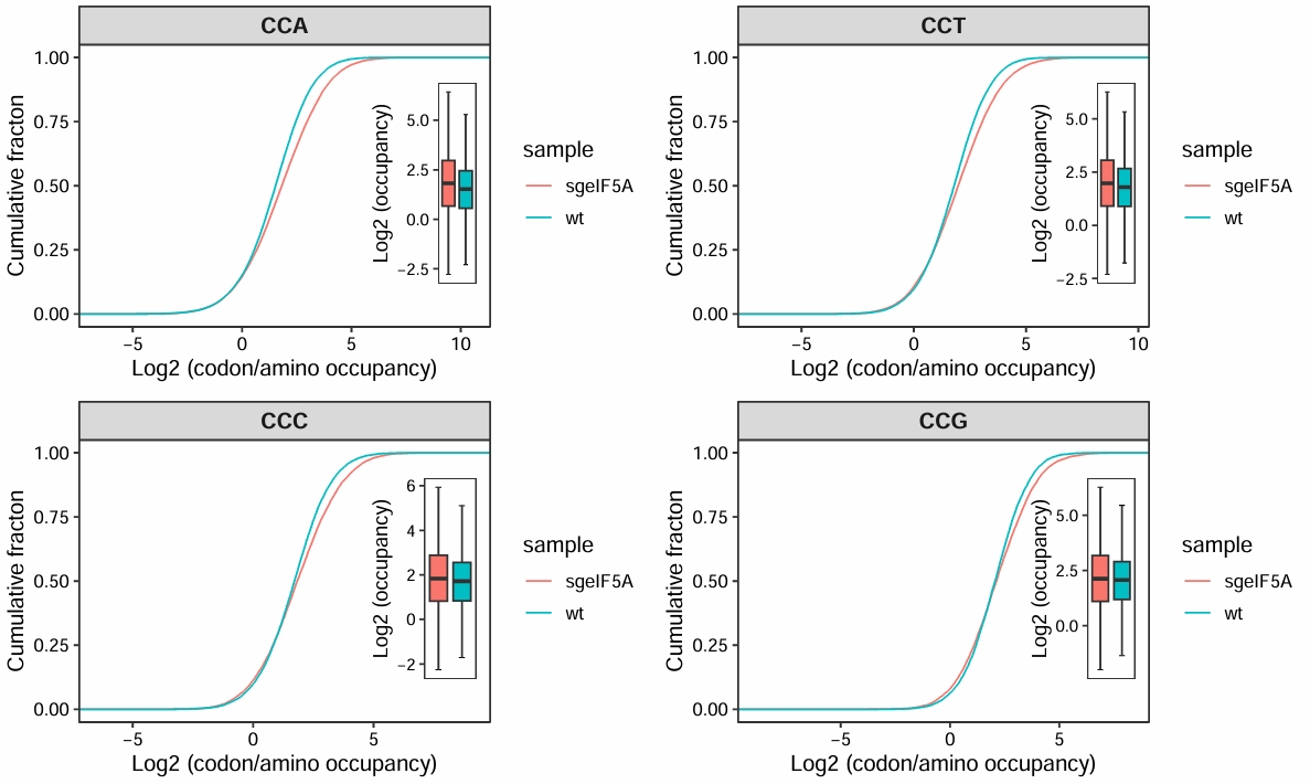
motif_occupancy(object = obj0,
                cds_fa = "./sac_cds.fa",
                search_type = "codon",
                do_offset_correct = T,
                motif_pattern = c("CCA","CCT","CCG","CCC"))
# `summarise()` has grouped output by 'sample', 'rname'. You can override using the `.groups` argument.
# Adding missing grouping variables: `sample_group`, `freq`
# $plot
#
# $statistics
# # A tibble: 24 × 9
# codon_seq .y.   group1       group2               p     p.adj p.format p.signif method
# <chr>     <chr> <chr>        <chr>            <dbl>     <dbl> <chr>    <chr>    <chr>
# 1 CCA       value sgeIF5A-rep1 sgeIF5A-rep2 2.36e-107 4.30e-106 < 2e-16  ****     Wilcoxon
# 2 CCA       value sgeIF5A-rep1 wt-rep1      2.32e-141 4.6 e-140 < 2e-16  ****     Wilcoxon
# 3 CCA       value sgeIF5A-rep1 wt-rep2      3.61e-  9 1.4 e-  8 3.6e-09  ****     Wilcoxon
# 4 CCA       value sgeIF5A-rep2 wt-rep1      0         0         < 2e-16  ****     Wilcoxon
# 5 CCA       value sgeIF5A-rep2 wt-rep2      2.80e-191 6.20e-190 < 2e-16  ****     Wilcoxon
# 6 CCA       value wt-rep1      wt-rep2      7.57e- 96 1.20e- 94 < 2e-16  ****     Wilcoxon
# 7 CCT       value sgeIF5A-rep1 sgeIF5A-rep2 5.02e- 99 8.50e- 98 < 2e-16  ****     Wilcoxon
# 8 CCT       value sgeIF5A-rep1 wt-rep1      4.70e- 62 5.6 e- 61 < 2e-16  ****     Wilcoxon
# 9 CCT       value sgeIF5A-rep1 wt-rep2      8.34e-  5 8.3 e-  5 8.3e-05  ****     Wilcoxon
# 10 CCT       value sgeIF5A-rep2 wt-rep1      0         0         < 2e-16  ****     Wilcoxon
# # ℹ 14 more rows
# # ℹ Use `print(n = ...)` to see more rows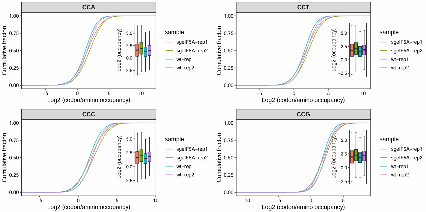
Merge replicates:
motif_occupancy(object = obj0,
                cds_fa = "./sac_cds.fa",
                search_type = "codon",
                do_offset_correct = T,
                merge_rep = T,
                motif_pattern = c("CCA","CCT","CCG","CCC"))
# `summarise()` has grouped output by 'sample', 'rname'. You can override using the `.groups` argument.
# $plot
#
# $statistics
# # A tibble: 4 × 9
# codon_seq .y.   group1  group2         p     p.adj p.format p.signif method
# <chr>     <chr> <chr>   <chr>      <dbl>     <dbl> <chr>    <chr>    <chr>
# 1 CCA       value sgeIF5A wt     1.85e-142 7.4 e-142 < 2e-16  ****     Wilcoxon
# 2 CCT       value sgeIF5A wt     3.55e- 53 1.10e- 52 < 2e-16  ****     Wilcoxon
# 3 CCC       value sgeIF5A wt     1.76e- 15 3.5 e- 15 1.8e-15  ****     Wilcoxon
# 4 CCG       value sgeIF5A wt     9.70e-  5 9.70e-  5 9.7e-05  ****     Wilcoxon