#!/usr/bin/env bash
ascp -QT -l 300m -P33001 -i $HOME/.aspera/connect/etc/asperaweb_id_dsa.openssh era-fasp@fasp.sra.ebi.ac.uk:vol1/fastq/SRR166/001/SRR1661491/SRR1661491.fastq.gz . && mv SRR1661491.fastq.gz rep1-SiControl-RPF.fastq.gz
ascp -QT -l 300m -P33001 -i $HOME/.aspera/connect/etc/asperaweb_id_dsa.openssh era-fasp@fasp.sra.ebi.ac.uk:vol1/fastq/SRR166/005/SRR1661495/SRR1661495.fastq.gz . && mv SRR1661495.fastq.gz rep2-SiControl-RPF.fastq.gz
ascp -QT -l 300m -P33001 -i $HOME/.aspera/connect/etc/asperaweb_id_dsa.openssh era-fasp@fasp.sra.ebi.ac.uk:vol1/fastq/SRR166/003/SRR1661493/SRR1661493.fastq.gz . && mv SRR1661493.fastq.gz rep1-SiYTHDF1_1-RPF.fastq.gz
ascp -QT -l 300m -P33001 -i $HOME/.aspera/connect/etc/asperaweb_id_dsa.openssh era-fasp@fasp.sra.ebi.ac.uk:vol1/fastq/SRR166/007/SRR1661497/SRR1661497.fastq.gz . && mv SRR1661497.fastq.gz rep2-SiYTHDF1_8-RPF.fastq.gz
ascp -QT -l 300m -P33001 -i $HOME/.aspera/connect/etc/asperaweb_id_dsa.openssh era-fasp@fasp.sra.ebi.ac.uk:vol1/fastq/SRR166/008/SRR1661498/SRR1661498.fastq.gz . && mv SRR1661498.fastq.gz rep2-SiYTHDF1_8-input.fastq.gz
ascp -QT -l 300m -P33001 -i $HOME/.aspera/connect/etc/asperaweb_id_dsa.openssh era-fasp@fasp.sra.ebi.ac.uk:vol1/fastq/SRR166/002/SRR1661492/SRR1661492.fastq.gz . && mv SRR1661492.fastq.gz rep1-SiControl-input.fastq.gz
ascp -QT -l 300m -P33001 -i $HOME/.aspera/connect/etc/asperaweb_id_dsa.openssh era-fasp@fasp.sra.ebi.ac.uk:vol1/fastq/SRR166/004/SRR1661494/SRR1661494.fastq.gz . && mv SRR1661494.fastq.gz rep1-SiYTHDF1_1-input.fastq.gz
ascp -QT -l 300m -P33001 -i $HOME/.aspera/connect/etc/asperaweb_id_dsa.openssh era-fasp@fasp.sra.ebi.ac.uk:vol1/fastq/SRR166/006/SRR1661496/SRR1661496.fastq.gz . && mv SRR1661496.fastq.gz rep2-SiControl-input.fastq.gz19 m6A modulates translation efficiency
19.1 Intro
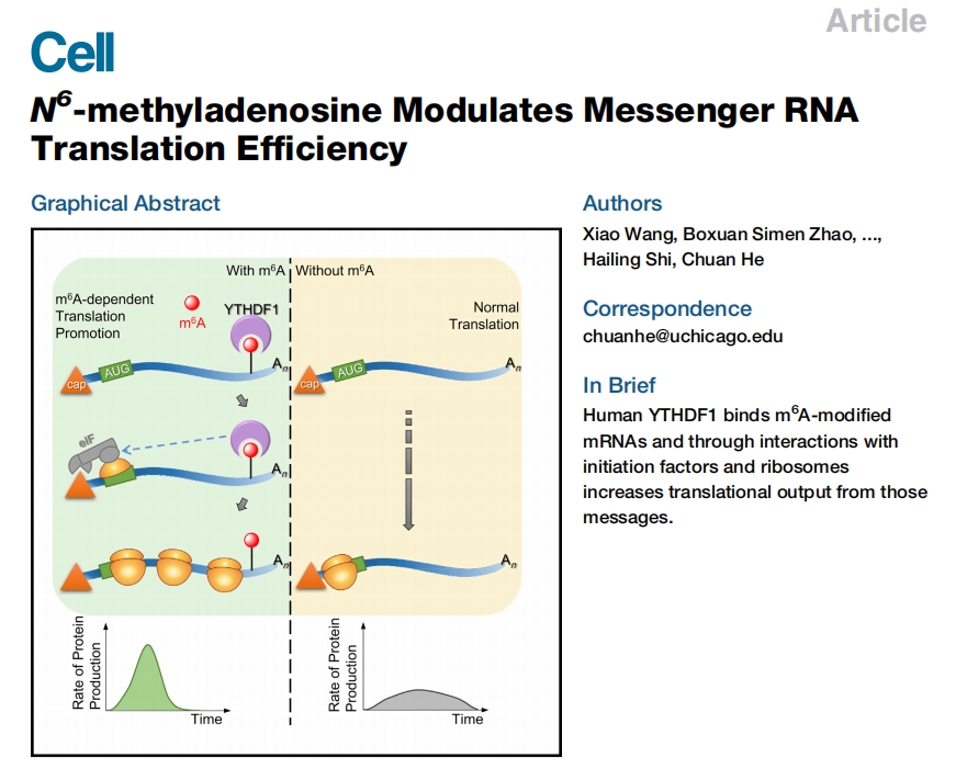
In this section, we reproduce key findings from a seminal 2015 Cell paper titled “N6-methyladenosine Modulates Messenger RNA Translation Efficiency.” Our focus centers on recreating the cumulative distribution curves that elegantly demonstrate how YTHDF1 knockdown affects both RNA stability and translational efficiency.
Cumulative distribution curves serve as powerful analytical tools in transcriptomic studies, providing comprehensive insights into the overall distribution characteristics of gene expression data. These curves are particularly valuable for visualizing global shifts in expression patterns and identifying systematic changes across entire transcriptomes.
19.2 Data download
First, we need to download the ribosome profiling (Ribo-seq) data from the original study. The data is deposited in the Gene Expression Omnibus (GEO) under accession number GSE63591:
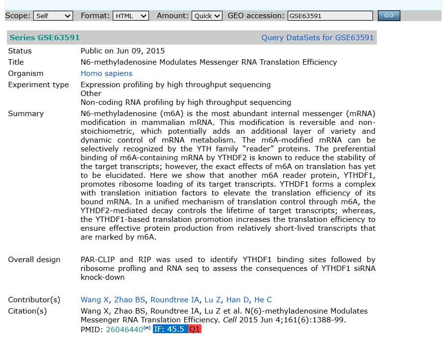
Download data by aspera:
19.3 Alignment to reference
After quality control assessment using FastQC software, the results indicated no adapter sequences were present in the data, allowing us to proceed directly to genome alignment. We performed genome alignment using HISAT2 with the following parameters:
for i in rep1-SiControl-input rep1-SiControl-RPF rep1-SiYTHDF1_1-input rep1-SiYTHDF1_1-RPF rep2-SiControl-input rep2-SiControl-RPF rep2-SiYTHDF1_8-input rep2-SiYTHDF1_8-RPF
do
    hisat2 -p 20 -x ../../index-data/grch38_hisat2_index/genome \
        --summary-file ${i}.mapinfo.txt \
        -U ../1.raw-data/${i}.fastq.gz \
        |samtools sort -@ 20 -o ${i}.sorted.bam
done

ls ./*.bam | xargs -i samtools index -@ 20 {}
19.4 Constructing the ribotrans object
Next, we construct RiboTrans objects from the aligned BAM files to facilitate downstream analysis of ribosome profiling data:
setwd("~/junjun_proj/34.ythdf1_ribo/2.map-data/")
getwd()


devtools::install_github("junjunlab/riboTransVis",force = TRUE)
library(riboTransVis)

gp <- c("siControl-rep1","siControl-rep2","siYTHDF1-rep1","siYTHDF1-rep2")

rnabams <- c("rep1-SiControl-input.sorted.bam",
             "rep2-SiControl-input.sorted.bam",
             "rep1-SiYTHDF1_1-input.sorted.bam",
             "rep2-SiYTHDF1_8-input.sorted.bam")

ribobams <- c("rep1-SiControl-RPF.sorted.bam",
              "rep2-SiControl-RPF.sorted.bam",
              "rep1-SiYTHDF1_1-RPF.sorted.bam",
              "rep2-SiYTHDF1_8-RPF.sorted.bam")

obj <- construct_ribotrans(gtf_file = "./Homo_sapiens.GRCh38.114.gtf.gz",
                           RNA_bam_file = rnabams,
                           RNA_sample_name = gp,
                           mapping_type = "genome",
                           assignment_mode = "end5",
                           Ribo_bam_file = ribobams,
                           Ribo_sample_name = gp,
                           choose_longest_trans = T)
19.4.1 QC for ribo-seq
Reads length and frames check:
# ==============================================================================
# QC
# ==============================================================================
obj <- generate_summary(object = obj,exp_type = "ribo", nThreads = 40)

length_plot(obj,type = "frame_length") +
  scale_fill_brewer(palette = "Greens",direction = -1)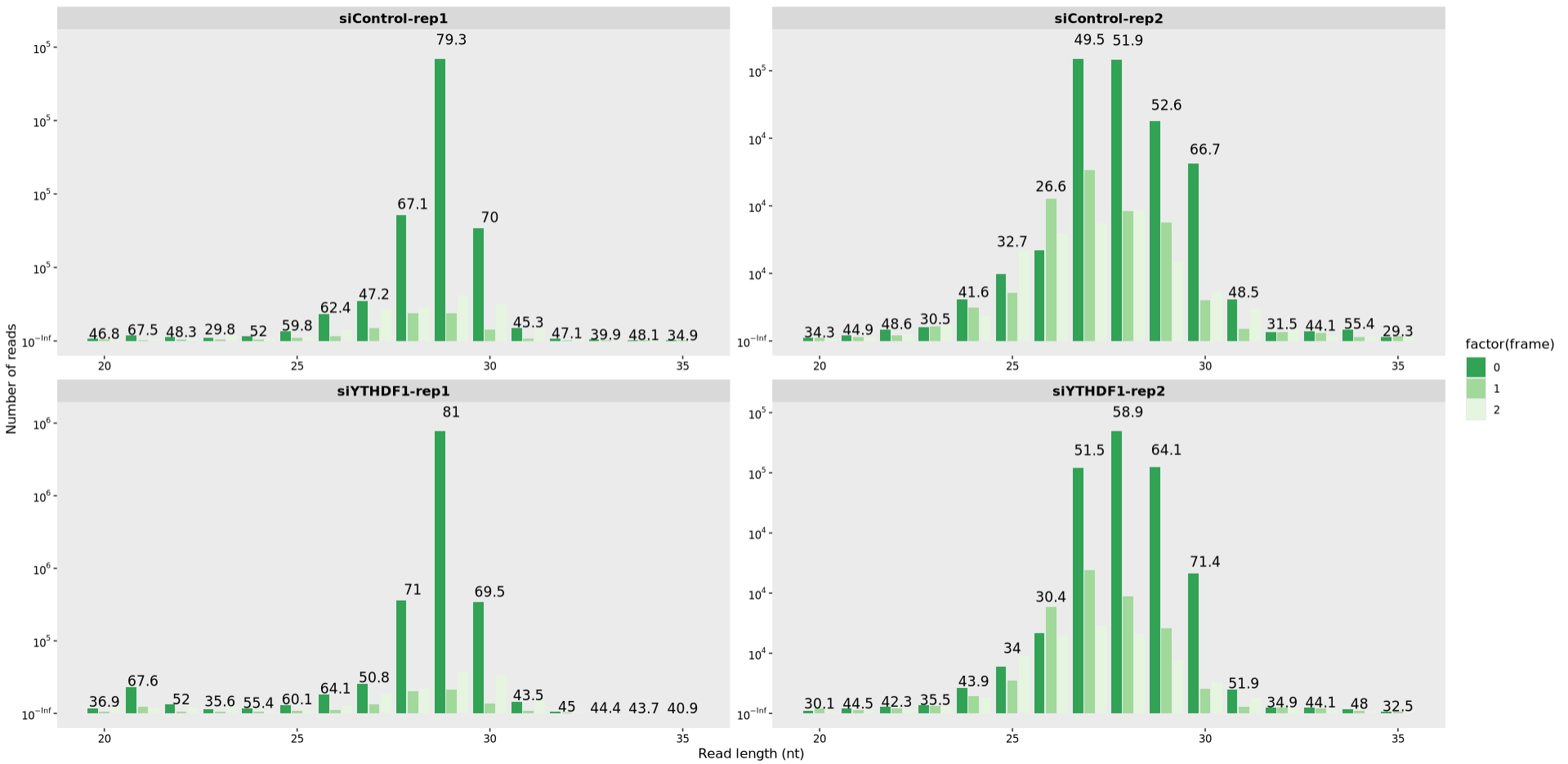
Offset check:
relative_offset_plot(obj)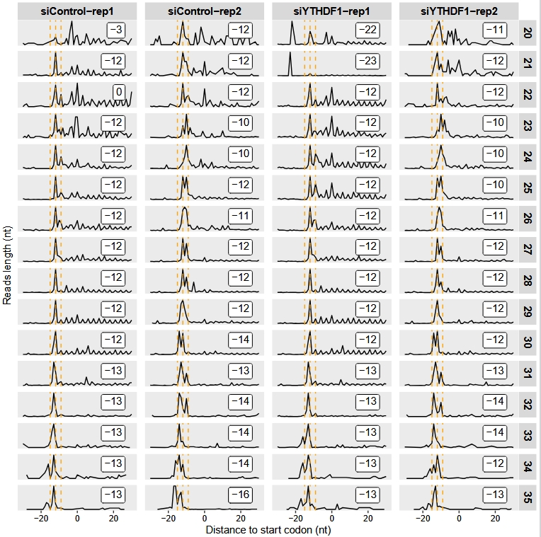
19.5 Reads counting
Counting reads for rna and rpf samples:
# ==============================================================================
# COUNT
# ==============================================================================

obj <- get_counts(obj, nThreads = 15)

# obj <- get_counts(obj, nThreads = 15, ribo_feature = "exon")

rna <- obj@counts$rna$counts
rpf <- obj@counts$rpf$counts

cc <- cor_plot(data = rna,x = "siControl-rep1",y = "siControl-rep2")
cy <- cor_plot(data = rna,x = "siYTHDF1-rep1",y = "siYTHDF1-rep2")

ccf <- cor_plot(data = rna,x = "siControl-rep1",y = "siControl-rep2")
cyf <- cor_plot(data = rna,x = "siYTHDF1-rep1",y = "siYTHDF1-rep2")

library(patchwork)
(cc + cy) / (ccf + cyf)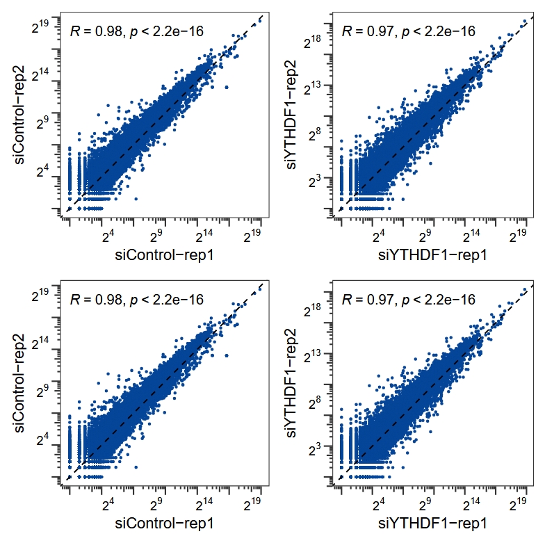
19.6 Differential analysis
Perform differential analysis separately for the RNA-seq (input), the Ribo-seq (RPF) and TE (translation efficiency). First, we download the information on YTHDF1 binding targets and non-binding targets provided by the paper and import it:
# ==============================================================================
# Differential analysis
# ==============================================================================
tt <- readxl::read_xlsx("1-s2.0-S0092867415005620-mmc2.xlsx",skip = 1)[,1:2] %>%
  na.omit()

colnames(tt) <- c("bind","gene")

# filter
tt <- tt %>%
  dplyr::filter(bind %in% c("CLIP only target","CLIP+IP target",
                            "Non-target"))

# check
table(tt$bind)
# CLIP only target   CLIP+IP target       Non-target
#             3652             1261             2822
RNA-seq differential analysis and plot cumulative curve:
# rna
diff.rna <- gene_differential_analysis(obj,
                                       type = "rna",
                                       control_samples = c("siControl-rep1",y = "siControl-rep2"),
                                       treat_samples = c("siYTHDF1-rep1",y = "siYTHDF1-rep2"))

# add binding type
diff.rna.anno <- diff.rna %>%
  dplyr::inner_join(y = tt,by = c("gene_name" = "gene"))


library(ggplot2)
library(ggsci)

# plot
ggplot(diff.rna.anno) +
  stat_ecdf(aes(x = log2FoldChange, color = bind)) +
  theme_bw() +
  theme(panel.grid = element_blank(),
        aspect.ratio = 1,
        axis.text = element_text(colour = "black")) +
  scale_color_manual(values = c("Non-target" = "grey50",
                                "CLIP only target" = "blue",
                                "CLIP+IP target" = "red"),
                     name = "Binding type")+
  xlim(-1.5,1.5) +
  ylab("Cumulative Fraction") +
  xlab("log2(siYTHDF1/siControl)\nmRNA Input")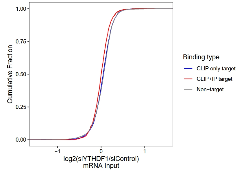
Ribo-seq (RPF) differential analysis and plot cumulative curve:
# rpf
diff.ribo <- gene_differential_analysis(obj,
                                        type = "ribo",
                                        control_samples = c("siControl-rep1",y = "siControl-rep2"),
                                        treat_samples = c("siYTHDF1-rep1",y = "siYTHDF1-rep2"))

# add binding type
diff.ribo.anno <- diff.ribo %>%
  dplyr::inner_join(y = tt,by = c("gene_name" = "gene"))

# plot
ggplot(diff.ribo.anno) +
  stat_ecdf(aes(x = log2FoldChange, color = bind)) +
  theme_bw() +
  theme(panel.grid = element_blank(),
        aspect.ratio = 1,
        axis.text = element_text(colour = "black")) +
  scale_color_manual(values = c("Non-target" = "grey50",
                                "CLIP only target" = "blue",
                                "CLIP+IP target" = "red"),
                     name = "Binding type") +
  xlim(-1.5,1.5) +
  ylab("Cumulative Fraction") +
  xlab("log2(siYTHDF1/siControl)\nRibosome bound fragments")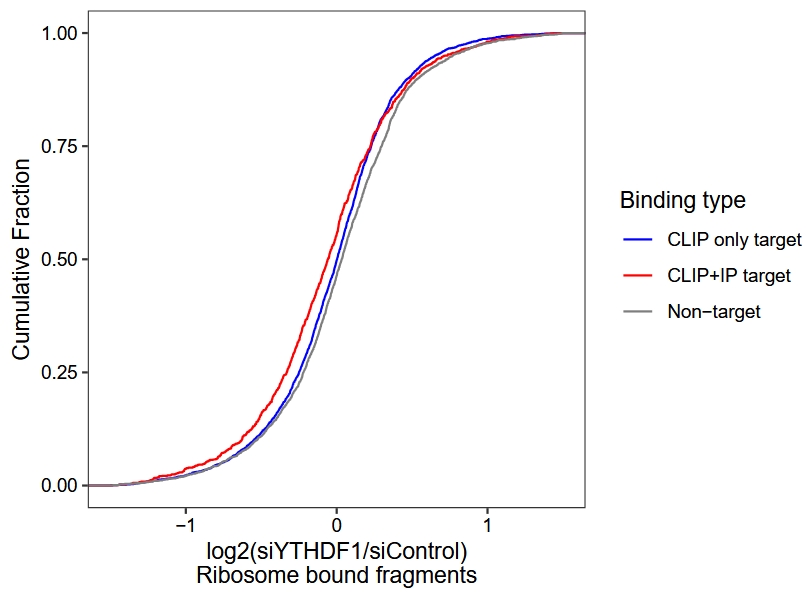
Translation efficiency (TE) differential analysis and plot cumulative curve:
# ==============================================================================
# te
# ==============================================================================

# use riborex for te analysis
te.rex <- TE_differential_analysis(object = obj,
                                   pkg = "riborex",
                                   control_samples = c("siControl-rep1",y = "siControl-rep2"),
                                   treat_samples = c("siYTHDF1-rep1",y = "siYTHDF1-rep2"))

te <- te.rex$deg_anno

# add binding type
diff.te.anno <- te %>%
  dplyr::inner_join(y = tt,by = c("gene_name" = "gene"))

# plot
ggplot(diff.te.anno) +
  stat_ecdf(aes(x = log2FoldChange, color = bind)) +
  theme_bw() +
  theme(panel.grid = element_blank(),
        aspect.ratio = 1,
        axis.text = element_text(colour = "black")) +
  scale_color_manual(values = c("Non-target" = "grey50",
                                "CLIP only target" = "blue",
                                "CLIP+IP target" = "red"),
                     name = "Binding type") +
  xlim(-1.5,1.5) +
  ylab("Cumulative Fraction") +
  xlab("log2(siYTHDF1/siControl)\nTranslation efficiency")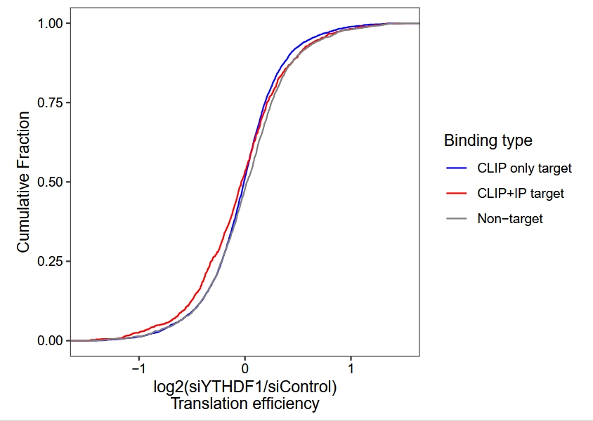
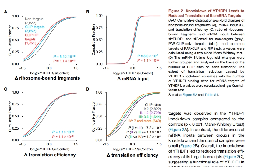
The following results is from original paper in figure 2:
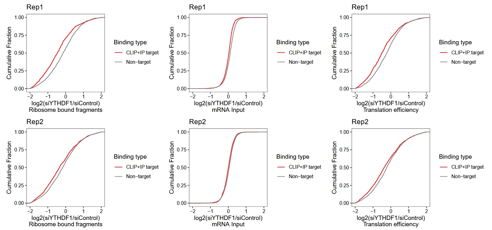
19.7 Cumulative curve for each replicate
The original paper also presented the distribution of ECDF (empirical cumulative distribution function) curves for RNA, RPF, and TE across individual biological replicates. Here, we need to obtain the normalized values for each sample, and then use the ratios between TE or RNA/RPF in siYTHDF1 and siControl to plot the cumulative distribution curves for each biological replicate:
# ==============================================================================
# normalized values
# ==============================================================================

norm <- get_normalized_reads(object = obj,
                             type = c("rna", "ribo", "te"))

# ==============================================================================
# rna

# add binding type
norm.rna <- norm$tpm.rna %>%
  dplyr::inner_join(y = tt %>% dplyr::filter(bind != "CLIP only target"),
                    by = c("gene_name" = "gene")) %>%
  dplyr::mutate(logrep1 = log2(`siYTHDF1-rep1`/`siControl-rep1`),
                logrep2 = log2(`siYTHDF1-rep2`/`siControl-rep2`))


# rna ecdf plot
rna.rep1 <-
ggplot(norm.rna) +
  stat_ecdf(aes(x = logrep1, color = bind)) +
  theme_bw() +
  theme(panel.grid = element_blank(),
        aspect.ratio = 1,
        axis.text = element_text(colour = "black")) +
  scale_color_manual(values = c("Non-target" = "grey50",
                                "CLIP+IP target" = "red"),
                     name = "Binding type")+
  xlim(-2,2) +
  ylab("Cumulative Fraction") +
  xlab("log2(siYTHDF1/siControl)\nmRNA Input") +
  ggtitle("Rep1")

rna.rep2 <-
  ggplot(norm.rna) +
  stat_ecdf(aes(x = logrep2, color = bind)) +
  theme_bw() +
  theme(panel.grid = element_blank(),
        aspect.ratio = 1,
        axis.text = element_text(colour = "black")) +
  scale_color_manual(values = c("Non-target" = "grey50",
                                "CLIP+IP target" = "red"),
                     name = "Binding type")+
  xlim(-2,2) +
  ylab("Cumulative Fraction") +
  xlab("log2(siYTHDF1/siControl)\nmRNA Input") +
  ggtitle("Rep2")

# ==============================================================================
# rpf

# add binding type
norm.rpf <- norm$tpm.ribo %>%
  dplyr::inner_join(y = tt %>% dplyr::filter(bind != "CLIP only target"),
                    by = c("gene_name" = "gene")) %>%
  dplyr::mutate(logrep1 = log2(`siYTHDF1-rep1`/`siControl-rep1`),
                logrep2 = log2(`siYTHDF1-rep2`/`siControl-rep2`))


# rpf ecdf plot
rpf.rep1 <-
  ggplot(norm.rpf) +
  stat_ecdf(aes(x = logrep1, color = bind)) +
  theme_bw() +
  theme(panel.grid = element_blank(),
        aspect.ratio = 1,
        axis.text = element_text(colour = "black")) +
  scale_color_manual(values = c("Non-target" = "grey50",
                                "CLIP+IP target" = "red"),
                     name = "Binding type")+
  xlim(-2,2) +
  ylab("Cumulative Fraction") +
  xlab("log2(siYTHDF1/siControl)\nRibosome bound fragments") +
  ggtitle("Rep1")

rpf.rep2 <-
  ggplot(norm.rpf) +
  stat_ecdf(aes(x = logrep2, color = bind)) +
  theme_bw() +
  theme(panel.grid = element_blank(),
        aspect.ratio = 1,
        axis.text = element_text(colour = "black")) +
  scale_color_manual(values = c("Non-target" = "grey50",
                                "CLIP+IP target" = "red"),
                     name = "Binding type")+
  xlim(-2,2) +
  ylab("Cumulative Fraction") +
  xlab("log2(siYTHDF1/siControl)\nRibosome bound fragments") +
  ggtitle("Rep2")

# ==============================================================================
# te
# add binding type
norm.te <- norm$te %>%
  dplyr::inner_join(y = tt %>% dplyr::filter(bind != "CLIP only target"),
                    by = c("gene_name" = "gene")) %>%
  dplyr::mutate(logrep1 = log2(`siYTHDF1-rep1`/`siControl-rep1`),
                logrep2 = log2(`siYTHDF1-rep2`/`siControl-rep2`))


# te ecdf plot
te.rep1 <-
  ggplot(norm.te) +
  stat_ecdf(aes(x = logrep1, color = bind)) +
  theme_bw() +
  theme(panel.grid = element_blank(),
        aspect.ratio = 1,
        axis.text = element_text(colour = "black")) +
  scale_color_manual(values = c("Non-target" = "grey50",
                                "CLIP+IP target" = "red"),
                     name = "Binding type")+
  xlim(-2,2) +
  ylab("Cumulative Fraction") +
    xlab("log2(siYTHDF1/siControl)\nTranslation efficiency") +
  ggtitle("Rep1")

te.rep2 <-
  ggplot(norm.te) +
  stat_ecdf(aes(x = logrep2, color = bind)) +
  theme_bw() +
  theme(panel.grid = element_blank(),
        aspect.ratio = 1,
        axis.text = element_text(colour = "black")) +
  scale_color_manual(values = c("Non-target" = "grey50",
                                "CLIP+IP target" = "red"),
                     name = "Binding type")+
  xlim(-2,2) +
  ylab("Cumulative Fraction") +
  xlab("log2(siYTHDF1/siControl)\nTranslation efficiency") +
  ggtitle("Rep2")


# combine
(rpf.rep1 + rna.rep1 + te.rep1) / (rpf.rep2 + rna.rep2 + te.rep2)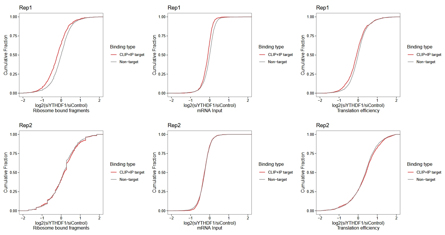
It can be seen that replicate 2 does not perform very well and is not quite consistent with the results reported in the original paper. The following results is from original paper in figure S2:
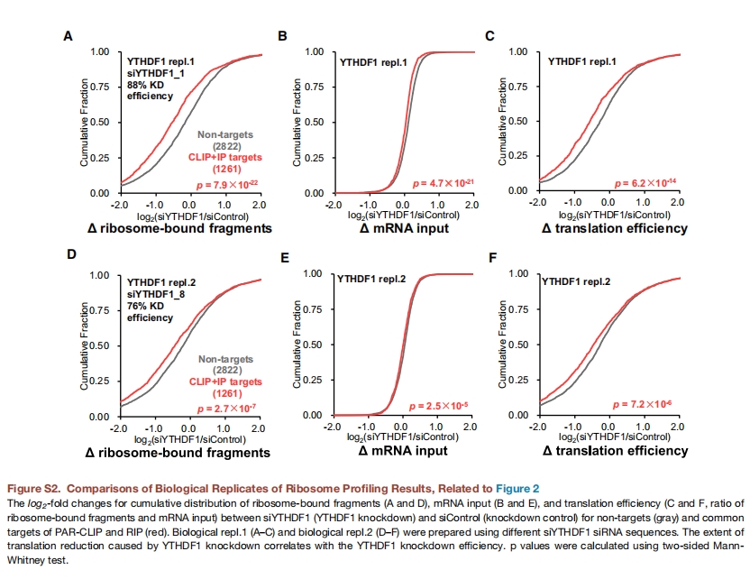
19.8 Using orignal data
We can use the pre-calculated data provided in the paper to replot the ECDF curves:
# ==============================================================================
# gse data
# ==============================================================================

dt <- read.csv("gse_siYTHDF1.csv") %>%
  dplyr::inner_join(y = tt %>% dplyr::filter(bind != "CLIP only target"),
                    by = c("Gene.symbol" = "gene"))

colnames(dt)
# [1] "Gene.symbol" "ribo.rep1"   "rna.rep1"    "te.rep1"     "ribo.rep2"   "rna.rep2"    "te.rep2"     "bind"

rna.rep1 <-
  ggplot(dt) +
  stat_ecdf(aes(x = rna.rep1, color = bind)) +
  theme_bw() +
  theme(panel.grid = element_blank(),
        aspect.ratio = 1,
        axis.text = element_text(colour = "black")) +
  scale_color_manual(values = c("Non-target" = "grey50",
                                "CLIP+IP target" = "red"),
                     name = "Binding type")+
  xlim(-2,2) +
  ylab("Cumulative Fraction") +
  xlab("log2(siYTHDF1/siControl)\nmRNA Input") +
  ggtitle("Rep1")

rna.rep2 <-
  ggplot(dt) +
  stat_ecdf(aes(x = rna.rep2, color = bind)) +
  theme_bw() +
  theme(panel.grid = element_blank(),
        aspect.ratio = 1,
        axis.text = element_text(colour = "black")) +
  scale_color_manual(values = c("Non-target" = "grey50",
                                "CLIP+IP target" = "red"),
                     name = "Binding type")+
  xlim(-2,2) +
  ylab("Cumulative Fraction") +
  xlab("log2(siYTHDF1/siControl)\nmRNA Input") +
  ggtitle("Rep2")

# rpf ecdf plot
rpf.rep1 <-
  ggplot(dt) +
  stat_ecdf(aes(x = ribo.rep1, color = bind)) +
  theme_bw() +
  theme(panel.grid = element_blank(),
        aspect.ratio = 1,
        axis.text = element_text(colour = "black")) +
  scale_color_manual(values = c("Non-target" = "grey50",
                                "CLIP+IP target" = "red"),
                     name = "Binding type")+
  xlim(-2,2) +
  ylab("Cumulative Fraction") +
  xlab("log2(siYTHDF1/siControl)\nRibosome bound fragments") +
  ggtitle("Rep1")

rpf.rep2 <-
  ggplot(dt) +
  stat_ecdf(aes(x = ribo.rep2, color = bind)) +
  theme_bw() +
  theme(panel.grid = element_blank(),
        aspect.ratio = 1,
        axis.text = element_text(colour = "black")) +
  scale_color_manual(values = c("Non-target" = "grey50",
                                "CLIP+IP target" = "red"),
                     name = "Binding type")+
  xlim(-2,2) +
  ylab("Cumulative Fraction") +
  xlab("log2(siYTHDF1/siControl)\nRibosome bound fragments") +
  ggtitle("Rep2")


# te ecdf plot
te.rep1 <-
  ggplot(dt) +
  stat_ecdf(aes(x = te.rep1, color = bind)) +
  theme_bw() +
  theme(panel.grid = element_blank(),
        aspect.ratio = 1,
        axis.text = element_text(colour = "black")) +
  scale_color_manual(values = c("Non-target" = "grey50",
                                "CLIP+IP target" = "red"),
                     name = "Binding type")+
  xlim(-2,2) +
  ylab("Cumulative Fraction") +
  xlab("log2(siYTHDF1/siControl)\nTranslation efficiency") +
  ggtitle("Rep1")

te.rep2 <-
  ggplot(dt) +
  stat_ecdf(aes(x = te.rep2, color = bind)) +
  theme_bw() +
  theme(panel.grid = element_blank(),
        aspect.ratio = 1,
        axis.text = element_text(colour = "black")) +
  scale_color_manual(values = c("Non-target" = "grey50",
                                "CLIP+IP target" = "red"),
                     name = "Binding type")+
  xlim(-2,2) +
  ylab("Cumulative Fraction") +
  xlab("log2(siYTHDF1/siControl)\nTranslation efficiency") +
  ggtitle("Rep2")


# combine
(rpf.rep1 + rna.rep1 + te.rep1) / (rpf.rep2 + rna.rep2 + te.rep2)